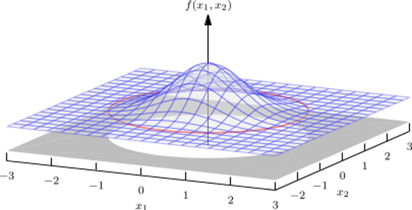
Today we talked about covariance and multivariate normal distributions. We started with the following warm-up problems:
Suppose that \(X_1, X_2\) are i.i.d. \(\operatorname{Norm}(0,1)\) random variables. What is the joint density function for the random vector \(X = (X_1,X_2)^T\)?
Let \(R = \begin{bmatrix} \cos \theta & - \sin \theta \\ \sin \theta & \cos \theta \end{bmatrix}\). Notice that \(R\) is rotation matrix for an angle of \(\theta\). Let \(Y = RX\) where \(X\) has the joint distribution above. What is the joint distribution function for \(Y\)?
Suppose \(X\) and \(Y\) are random variables with respective means \(\mu_X\) and \(\mu_Y\). The covariance of \(X\) and \(Y\) is \[\operatorname{Cov}(X,Y) = E((X-\mu_X)(Y-\mu_Y))\]
Suppose \(X_1, X_2\) and \(Y\) are random variables and \(a, b\) are constants. Then, \[\operatorname{Cov}(aX_1 + b X_2,Y) = a \operatorname{Cov}(X_1,Y) + b \operatorname{Cov}(X_2,Y).\]
Suppose \(X\) and \(Y\) are random variables, then \[\operatorname{Cov}(X,Y) = \operatorname{Cov}(Y,X).\]
Suppose \(X\) and \(Y\) are independent random variables, then \(\operatorname{Cov}(X,Y) = 0\).
Notice, this is not an if and only if theorem. The converse is not always true.
You can also talk about the covariance of random vectors.
Suppose that \(X = \begin{bmatrix} X_1 \\ \vdots \\ X_n \end{bmatrix}\) is a random vector with entry-wise means \(\mu_X = \begin{bmatrix} \mu_{X_1} \\ \vdots \\ \mu_{X_n}\end{bmatrix}\). The covariance matrix for \(X\) is \[\Sigma_X = \begin{bmatrix} \operatorname{Cov} (X_1, X_1) & \ldots & \operatorname{Cov} (X_1, X_n) \\ \vdots & & \vdots \\ \operatorname{Cov} (X_m, X_1) & \ldots & \operatorname{Cov} (X_m, X_n) \end{bmatrix}.\]
Observe that the entry in row \(i\), column \(j\) of the covariance matrix is the covariance of \(X_i\) and \(X_j\):
It is not hard to show that covariance matrices have the following linearity property:
Suppose that \(X\) is a random vector and \(A\) is a matrix of the right size so that \(AX\) makes sense. Then \[\operatorname{Cov}(AX,AX) = A \operatorname{Cov}(X,X) A^T.\]
A random vector \(X = (X_1, \ldots, X_n)^T\) has a multivariate normal distribution if the joint density function for \(X\) is \[f_X(x) = \frac{1}{(2\pi)^{n/2} |\Sigma|^{1/2}} \exp \left( -\tfrac{1}{2}(x-\mu_X)^T\Sigma^{-1}(x-\mu_X) \right).\] where \(\mu_X\) is the vector of entry-wise means for \(X\) and \(\Sigma\) is the covariance matrix of \(X\) (and \(|\Sigma|\) is the determinant of \(\Sigma\)). The parameters for a multivariate normal distribution are the vector \(\mu_X\) and the covariance matrix \(\Sigma\). These completely determine the joint distribution function.
If \(\Sigma\) is the \(n\)-by-\(n\) identity matrix and \(\mu_X = 0\), then \(X\) has the standard multivariate normal distribution: \[f_X(x) = \frac{1}{(\sqrt{2\pi})^n} e^{-\frac{1}{2} \|x \|^2}.\]
Today we will look at some applications of Multivariate Normal Distributions (MVNs). Recall that a MVN distribution can be completely described by two pieces of information: the vector of means \(\mu_X\) and the covariance matrix \(\Sigma_X\).
If a random vector \(X = (X_1, \ldots, X_n)^T\) has a multivariate normal distribution with vector of means \(\mu_X\) and covariance matrix \(\Sigma_X\), and \(A \in \mathbb{R}^{m \times n}\) is any matrix, then the random variable \(Y = AX\) has a multivariate normal distribution with mean \(\mu_Y = A\mu_X\) and covariance matrix \(\Sigma_Y = A \Sigma_X A^T\).
Remark: We didn’t prove this theorem, but the proof when \(A\) is invertible is one of this week’s homework problems. The theorem is still true, even if \(A\) is not invertible, but that is a little harder to prove.
If \(X_1, \ldots, X_n\) are i.i.d. normal random variables with mean \(\mu\) and variance \(\sigma^2\), and \(a, b \in \mathbb{R}^{n \times n}\), then \(a^T X\) and \(b^T X\) are independent random variables if and only if \(a\) and \(b\) are orthogonal.
Suppose \(X_1, \ldots X_n \sim \operatorname{Norm}(\mu, \sigma)\) are i.i.d. RVs. What is the covariance matrix for the random vector \(X\)?
Suppose that \(X_1, \ldots X_n \sim \operatorname{Norm}(\mu, \sigma)\) are i.i.d. RVs. Show that the average value \(\bar{x}\) is independent of \(X_i - \bar{x}\) for every \(i\).
An immediate consequence is the following result.
If \(X_1, \ldots, X_n\) is a random sample of \(N\) independent observations chosen from a population with a normal distribution, then the sample mean \(\bar{x} = \frac{1}{n}(X_1 + \ldots + X_n)\) and the sample variance \(s^2 = \frac{1}{n-1} \sum_i (X_i-\bar{x})^2\) are independent random variables.
Today we defined the \(\chi^2\)-distribution and we used it to explain why you divide by \(n-1\) instead of \(n\) in the formula for the sample variance.
Suppose that \(X\) is a random vector whose entries \(X_1, \ldots, X_n\) are independent \(\operatorname{Norm}(0,1)\) random variables. The \(\chi^2\)-distribution with \(n\) degrees of freedom is the probability distribution for $|X |^2.

Suppose that \(X\) is a random vector whose entries \(X_1, \ldots, X_n\) are independent \(\operatorname{Norm}(\mu,\sigma)\) random variables and \(P \in \mathbb{R}^{n \times n}\) is an orthogonal projection matrix. Then \(\frac{1}{\sigma^2} \|PX\|^2\) has a \(\chi^2\) distribution with degrees of freedom equal to the dimension of \(\operatorname{Range}(P)\).
We didn’t try to prove this theorem, but if we have time later in the semester we might come back to it. As an application of this theorem, consider the sample variance of a collection of independent observations \(X_1, \ldots X_n\) from a normal distribution with mean \(\mu\) and variance \(\sigma^2\):
\[s^2 = \frac{1}{n-1} \sum_{i = 1}^n (x_i - \bar{x})^2.\] The expression \(\sum_{i = 1}^n (x_i - \bar{x})^2 = \| (I - \frac{1}{n} ee^T) X \|\) and we proved in Homework 3, Problem 2 that \(I-\frac{1}{n}ee^T\) is an orthogonal projection.
What is the nullspace of \(I - \frac{1}{n}ee^T\). Hint: show that a vector \(v \in \mathbb{R}^n\) is in \(\operatorname{Null}(I-\frac{1}{n}ee^T)\) if and only if all of the entries of \(v\) are the same.
Use the Fundamental Theorem of Linear Algebra to show that the dimension of \(\operatorname{Range}(I-\frac{1}{n}ee^T) = n-1\).
From this, we can see that \(s^2\) is \(\frac{\sigma^2}{n-1}\) multiplied by a random variable with a \(\chi^2(n-1)\) distribution.
Suppose that \(s^2\) is the sample variance of \(n\) independent observations from a normal distribution with mean \(\mu\) and standard deviation \(\sigma\). Then \[\frac{(n-1)s^2}{\sigma^2}\] has a \(\chi^2\)-distribution with \(n-1\) degrees of freedom.