Today we continued talking about partial derivatives. For the first part of the class, we focused on the meaning of the partial derivative as a rate of change in the output as each input changes. When \(z = f(x,y)\), this leads to the formula:
\[\Delta z = \frac{\partial f}{\partial x} \Delta x + \frac{\partial f}{\partial y} \Delta y.\]
We did the following examples:
The distance formula \(d(x,y) = \sqrt{x^2+y^2}\) finds the distance from a point \((x,y)\) to the origin. It is easy to calculate \(d(6,8) = 10\). Find the partial derivatives of \(d\) at \(x = 6\) and \(y = 8\), and use them to estimate the value of \(d(6.2,7.9)\).
Suppose that a factory has hourly output \(Q(K,L) = 30 K^{0.3} L^{0.7}\) where \(K\) is capital expenditures (in dollars) and \(L\) is labor (number of workers). Find the marginal productivity of capital and the marginal productivity of labor when \(K = 600\) and \(L = 600\).
A cylindrical can has surface area \(S = 2\pi r^2 + 2 \pi r h\). Find the partial derivatives \(S_r\) and \(S_h\). If the dimensions of the cylinder are \(r=2\)cm and \(h = 10\)cm, then which would have a greater affect on surface area: increasing the height by 1cm or increasing the radius by 1cm?
We finished with the following idea: For a function \(f(x,y)\), the two partial derivatives give the direction of steepest ascent. From any point \((x,y)\), if you move \(\dfrac{\partial f}{\partial x}\) steps horizontally and \(\dfrac{\partial f}{\partial y}\) steps vertically, that is the direction of steepest ascent. The direction of steepest ascent is always perpendicular to the level curves.
Today we talked about how to find the max or min of a function with two variables. Since there are two partial derivatives, you have to set them both equal to zero to find the critical points. We started with these two examples.
\(z = 6x+8y - x^2 - y^2\).
\(f(x,y) = x^3+y^3+3x^2-3y^2+1\).
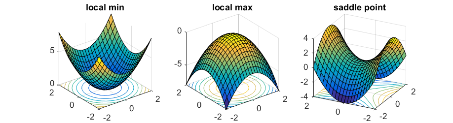
Example 2 had four critical points. Which raises the question, how do you know whether critical points are maximums or minimums? It turns out two of the critical points are neither: they are saddle points. There are three types of critical points for two variable functions:
To tell the difference you need to calculate the 2nd partial derivatives. Then you calculate the determinant:
\[D = f_{xx} \cdot f_{yy} - (f_{xy})^2.\]
The Second Derivative Test for Two Variable Functions says:
We went back and used this 2nd Derivative Test on both example 1 and example 2 above. Then we did the following additional examples:
Find the 2nd derivatives of \(f(x,y) = e^x y^3\). (We did this example to show that the mixed 2nd partial derivatives \(f_{xy}\) aren’t always zero.)
Find the critical point(s) of \(z = x^2 + 2y^2 - xy + 14y\) and use the 2nd derivative test to see if they are max/mins/ or saddle points.
In example 4 above, you need to solve two equations for two unknowns. To solve two equations with two unknowns, use one equation to make a substitution that eliminates one of the variables in the other equation. We used this same idea in this example too:
A company makes two products. The demand equations for the two products are given below where \(x\) and \(y\) are the prices the company chooses for product 1 and product 2 respectively. \[Q_1=200-3x-y\] \[Q_2=150-x-2y\] Find the price the company should charge for each product in order to maximize total revenue. What is that maximum revenue?
Notice that \(\partial Q_1/\partial y = -1\) and \(\partial Q_2/\partial x = -1\). What does this mean about product 1 and product 2? Are they complimentary or substitute goods?
Today we introduced the method of Lagrange multipliers. To maximize (or minimize) a function \(f(x,y)\) subject to a constraint \(g(x,y) = k\), you want the direction of steepest ascent for \(f\) to match the direction of steepest ascent for \(g\). This leads to three equations that you can solve for the three unknowns \(x, y\), and \(\lambda\):
\[f_x = \lambda g_x ~~~~~ f_y = \lambda g_y ~~~~~ g(x,y) = k.\]
These are called the Lagrange multiplier equations and \(\lambda\) is called the Lagrange multiplier. We did the following examples together in class:
Maximize \(f(x,y) = 3x+4y\) subject to the constraint \(g(x,y) = x^2 + y^2 = 25\).
600 meters of fence are use to fence off 3 sides of a rectangular field along the side of a river. What dimensions maximize the area of the rectangle?
Postal regulations say the length plus the circumference of a cylindrical package sent by 4th class mail cannot exceed 9 feet. What dimensions of the cylinder maximize volume?