LABORATORY EIGHT

NATURAL SELECTION AND GENE FREQUENCIES

OBJECTIVES OF LABORATORY:

• To explore the process of natural selection.

• To demonstrate the concepts of normal distribution and continuous variation.

• To explore the effects of environment on gene frequencies within populations.

• To investigate lethal recessive alleles and the factors that determine their frequency.

PART I: Modeling Natural Selection

            The moth species, Biston betularia, known as the peppered moth for its lightly mottled, speckled coloration, blends perfectly with lichen-covered bark. This coloration serves as an ideal camouflage from birds and other predators.  The moths blend in so well that they are nearly impossible to distinguish from the tree trunks on which they rest during the day.  But the coloration of this species is not uniform; lighter and darker forms, or morphs, exist, including some individuals that are almost black.  The latter stand out so well against a light-colored background that they are easily picked off by birds.  The black moths are so rare that the first was not captured until 1848, and then made up only a tiny proportion of the population.

            Although the lighter moths were well adapted, the environment pulled a fast one on them. Smoke and soot began pouring out of new factories during Great Britain's Industrial Revolution in the mid-19th century, killing the lichens and settling on the tree trunks, turning them a grimy black.  Suddenly the darker moths possessed the advantage; the lighter individuals were now conspicuous and more prone to predation.  By 1880 many melanistic, darkly pigmented, moths were observed around London and other industrialized areas, particularly northern cities such as Manchester, Liverpool, Birmingham, and Leeds.  By the turn of the century the white moths were totally outnumbered and now constituted a mere one percent of the population.  In just a few decades the moth population changed from predominantly lighter to predominantly darker morphs — in other words, the population evolved.

            Several British biologists, including E.B. Ford and later H.B.D. Kettlewell, both of Oxford, reasoned that natural selection accounted for the change.  Do you think they were correct?  How might they have tested their hypothesis?  One method often used by biologists to test whether a hypothesis seems reasonable is to model the process the hypothesis seeks to explain.  These models are not like airplanes or trains but rather simple systems or situations that mimic more complex situations.  Models are very useful tools, but it is important to keep in mind that they do not represent the actual situation.  They almost always contain simplifications and inaccuracies that must be considered when evaluating the experimental results. How could a model be used to test Ford and Kettlewell’s hypothesis that natural selection accounted for changes in moth coloration?  That is what you will determine in this lab.

Procedure:

1.         If you and your partner have a dark environmental tray, take a set of moths.  If your tray has a green background, take a set of squares.  Each set of moths contains 59 moths in nine varying intensities, from white to black (in the ratio 3: 4: 7: 10: 11: 10: 7: 4: 3, with 11 gray moths).  Each set of squares contains 82 squares in seven sizes, starting at ½ " and increasing by ¼ " to 2" (in the following quantities:  5: 10: 17: 18: 17: 10: 5).

2.         Arrange the moths or squares so that you can study the range of colors or sizes.

3.         One member of each pair should place the moths or squares into the tray and stir them to spread them out evenly over the surface.

4.         While scanning the tray, the other student should quickly select five obvious, conspicuous moths or squares, one at a time, and set them aside.  Do not select randomly; pick the moths or squares that stand out.

5.         One student in each pair will record which five moths or squares were selected.  Place a tick mark in the appropriate box on the data chart found on page 8-11 to tally the moths or squares that you draw from the model environment.

 6.        Place the chosen moths or squares back in the box, stir again, and repeat the selection and recording steps.  Perform this simple process ten times.

Analysis:  Write the answers to these questions on lined paper and attach the page to your answer sheet.  Make sure that you number your answers.  You will hand in your answers at the end of the lab.

1.         What distribution do the ranges of moth colors and square sizes represent?  What type of variation do they represent?  See page 8-8 for helpful suggestions. Answer question #2 and/or #3, depending on your instructor’s directions.

2.         For your moth selection data, add up all the numbers on either side of the middle number; do not include the middle number for the gray moths in your count.  Did you select more light-colored moths or dark-colored moths?  How do you explain this? 

3.         Examine your square selection data, and again add up all numbers on either side of the middle number for the 1 ¼ " squares.  Did you select more small or large squares? 

4.         List a few other possible factors, aside from body size and color that might make moths more conspicuous or preferentially selected by predators.  Think about moth behavior, for example.  What if birds did not detect moths visually?

5.         Giraffes eat leaves high up on trees.  Is it a coincidence that they have long necks?  Do you think some giraffes might have shorter necks?  What happens to them? 

6.         If your dog has learned new tricks (e.g., leaping for frisbees), will her puppies have an advantage (i.e., be better than the average dog) in these games?  Why or why not?

7.         Describe the components of this model (e.g., what does the tray represent; the squares, the predator, etc.?). In what ways is this model accurate and inaccurate in its depiction of natural selection?

2.         To simulate mating, shake the collected beads to mix them, and then tip the tray to allow a line of beads to collect at the front. These represent your first generation of offspring organisms.  Your instructor will demonstrate this process.

3.         Starting at one end, count off the beads in pairs.  Remember that each organism has two alleles for each gene, thus 100 beads = 50 individuals.  As you count, note that any organism possessing two red beads has a lethal combination — it would not survive.  Simulate its death by removing that pair of red beads from the gene pool (i.e., removing that homozygous recessive individual from the population).

4.         Determine the number of beads remaining in the gene pool and calculate the new percentage of recessive (red) alleles. Do this by dividing the number of red beads remaining by the new total number of beads. Record and plot this value in the table and graph in the row labeled Generation 1.

5.         The survivors now reproduce to start the next generation. Assume that the population size holds constant at 50 individuals (100 gene pairs). However, because natural selection has eliminated some of the recessive lethal alleles (red beads), you must adjust the frequency of the recessive allele so the new frequency appears in the new generation. To simulate this, add a sufficient number of white (or non-red) beads to your tray to reset the gene frequency to the value calculated in Step 4. For example, if the value you plotted in Step 4 was 14% and you had 96 total alleles remaining, add 4 white beads so that your new population has 14 red beads and 86 white (a total of 100).

6.         Repeat Steps 2-5 for ten generations, and graph your results.

7.         Compare your plotted curve with that of other groups.  How are they similar?  How do they differ?

Analysis:

1.         Write a paragraph that links the manipulations in this simulation (or model) with the natural processes they were intended to simulate (e.g., what do the beads represent? Why did you mix the beads? etc.).

2.         What effect does natural selection have on the frequency of lethal recessive alleles in a population? Are such alleles completely eliminated? Defend your answers using the data you collected.

3.         In what ways is this model accurate and inaccurate in its depiction of natural selection and the movement of genes within populations?

PART III: Modeling Natural Selection, Gene Frequency, and Mutation

            After you have finished the bead exercise and drawn some tentative conclusions, you will evaluate further how natural selection affects gene frequencies.  This will help you, in particular, to determine whether your answer to the second Analysis question was correct.  Just as with the beads, the computer simulation will eliminate organisms that possess pairs of lethal recessive alleles, which in turn influences which individuals will reproduce and pass their genes on to the next generation.  A computer program called NATSELPC allows us to simulate natural selection more realistically and easily than the bead exercise by allowing us to observe much larger populations over many more generations.

            NATSELPC offers many other advantages as well.  It allows us to handle smaller gene frequencies, which in real life seldom exceed 5% for truly lethal recessives.  It plots data in a form that can be easily printed and analyzed.  It also can simulate the effect of mutations, changes in genes that can convert normal alleles into recessive lethal alleles.  Mutations can have the effect of continually replacing lethal recessive genes even as natural selection removes them from a population.

            Thus natural selection and mutation act as opposing forces that control gene frequency by reaching a stable yet dynamic equilibrium.  NATSELPC allows us to change both the force of selection and the rate of mutation in order to study how the two interact to produce an equilibrium frequency for the gene in question.  To simplify things, we will hold the force of selection at 100% in all the simulations described in this exercise (that means that all of the recessive homozygotes die without reproducing—in other words, the recessive allele is lethal).

            NATSELPC produces a graph of the frequency of the lethal allele versus the generation number just like the simple graph you drew earlier.  Although the frequency of an allele may approach zero on the screen, don't consider it eliminated without checking the final frequency, which appears below the graph.  The allele is eliminated only if this number is zero. (In some of your simulations, you will note that even without mutation, the allelic frequency stabilizes at a very low, non-zero level.  Think about why this might happen.)

            Note:  You will learn the most from NATSELPC if you only change one variable at a time.  That way, any change in your graph can reliably be attributed to the change you made in that single variable.

Procedure:

1.      NATSELPC is available on our laboratory Dell computers, in a folder entitled Biology 151, or, simply NATSEL.  Begin by opening this folder, then the program NATSELPC.  Follow the on-screen directions.  Remember to press "enter" after any typed commands.  Each of the parameters (population size, number of generations, etc.) can be altered, but each has a default value—a value that the program uses if you do not indicate otherwise.  These values are listed in the following chart:

                                    Population size            1000

                                    Percent recessive         20

                                    Mutation rate              0

                                    Generations                 100

                                    Selection rate              100

The program will not accept a population size larger than 10,000, mutation rates less than zero, or selection rates higher than 100.

2.         Repeat your bead exercise with NATSELPC.  The values you will use are different from the default values in the chart, so be sure that you change them to correspond to the bead exercise.  First, set population size to 50, and enter.  Next, set the percent recessive to your assigned value (remember, don’t use a percent sign or convert the percent to a decimal value).  Leave mutation rate at the default value of zero.  Set generations to 10.  Leave the selection rate at the default value of 100 (100%; that means the recessive gene is lethal when homozygous).  DO NOT SELECT “RUN SIMULATION” UNTIL YOU HAVE COMPLETED THE NEXT STEP.

3.         You will eventually want to print out hard copies of your graphs, so at this point prepare a file to save them in. You will use several graphs to complete the Analysis, and you need to hand them in with your answers.

                        A. Select 6 (open text file) from the menu in the program, and enter.

                        B. Your graph file should appear on the desktop with your initials as the first 2 or 3 letters of the file name.  From now on, all of your graphs will go to this file.

            Now choose “run simulation” from the menu.  The graph generated by the simulation will appear on the screen, and will also be saved to your file.  Continue your analyses according to the instructions below.  You are automatically saving your graphs to the file that you named earlier, and you will print all of the graphs at once when you are finished with all the analyses. 

4.         Repeat the same simulation from Step 2, but increase the population to 5000. Note any changes from Step 3.

5.         Keep the population size at 5000, but run the simulation with 50 generations, then 100.

6.         Keep the population size at 5000, the number of generations at 50, and perform two additional simulations: one with an allele frequency much higher than your original and the second with an allele frequency much lower. 

7.         Set the allele frequency to 30%; keep the population at 5000 and generations at 50.  Run the simulation, and then repeat with a mutation rate of 5%.  Note any differences in the two graphs.

8.         Leave the mutation rate at 5%, but experiment with different allele frequencies.  What happens to the final frequency as you change starting frequencies?  Try changing the mutation frequency to see what happens.  If you are particularly adventurous, you might also try changing the selection value.  Your goal in this part of the exercise is to determine which parameters affect the final allele frequency when mutation is greater than zero.  If you don’t understand how to do this, ask your instructor.

To print your graphs

            Close the NATSELPC window.  Find your notepad file on the desktop; the first two or three letters of the file name will be the initials you entered at the very beginning.  The icon will look like a small notepad.  Open this file.  Using the scroll bar, check to make sure that all the graphs you want are there.  Any unwanted graphs can be highlighted and deleted, just as you would do in a word-processing program. While in this program, select all and copy to a word document.  There change the font size to 8, add a title and your names, and create page breaks after each graph to make it more readable. When you are sure that you have all the graphs you need, select “Print” from the File Menu at the top of the window. 

Analysis:

1.         Are the results from your computer simulation of the bead experiment (Step 2) similar to results obtained from the actual bead experiment (e.g., comparing changes in allele frequency and the final allele frequency)? If not, explain why they may be different.

2.         How does a population size of 5000 affect your results in Step 4?

3.         What effect does increasing the number of generations to 50 and 100 have on your results (Step 5)?

4.         What effect does decreasing and increasing the allele frequency have on your results (Step 6)? Write a general statement explaining the relationship between the starting and final gene frequencies of recessive lethal alleles after many generations of natural selection in the absence of mutation.

5.         What effect did mutation rates of 0% and 5% have on allele frequency when the starting frequency was 30%? (i.e., what effect does mutation rate have on the final allele frequency?) Which of the parameters (mutation rate, selection rate, starting allele frequency, number of generations, population size) affect the final frequency, and which do not?  Can you explain why?

6.         From what you have discovered about gene frequency, mutation rates, and natural selection, what is the likelihood of completely eliminating a recessive lethal gene from a large population? Explain.

Assignment:

1.         Answer all of the Analysis questions on separate loose-leaf paper. Be sure to label the part I, II, or III and the question number clearly. For the answers to Part 3, turn in the graphs that support your answers. Each team will submit only one set of graphs, but each team member will hand in his own answers.

2.         Read Lab 9, The Kingdoms of Monera and Protista.

Supplemental Information about Evolution and Variation

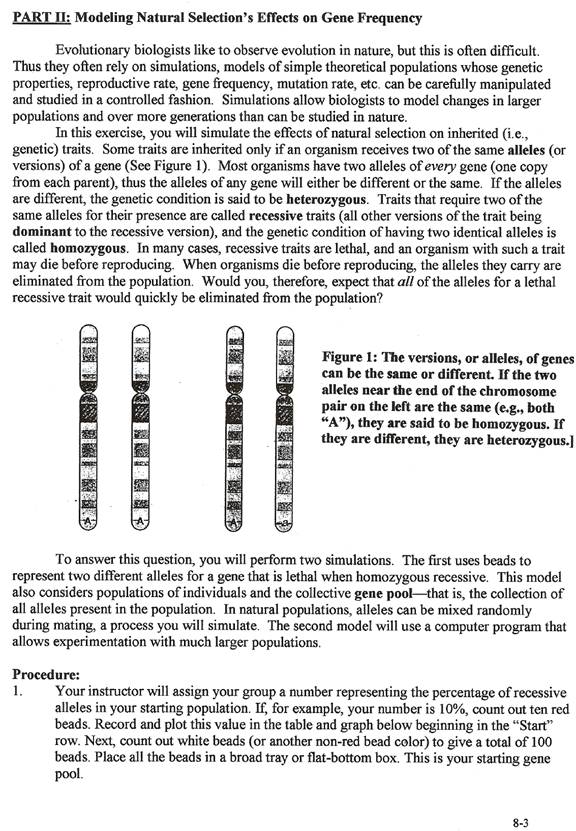
            It is a popular misconception that Charles Darwin first proposed the theory of evolution.  Indeed, many influential biologists before Darwin had considered, and adopted, the obvious concept of organic evolution, the idea that species are modified over time, or go extinct, while new species spring into existence from others.  Yet while there was substantial natural evidence to support the theory of evolution (in the fossil record, comparative anatomy, embryology, biogeography, and so forth), there was no understanding of the means by which it occurred.  Darwin's immortal contribution was the proposal of a mechanism for evolutionary change, which he designated natural selection.  Incidentally, Alfred Wallace, working independently of Darwin, conceived the idea of natural selection at the same time, although he did not publish his work.  Natural selection's influence on the course of evolution is no less impressive than Darwin's incontrovertible influence on the course of biology.

            The essence of evolution is descent with modification, and, if change is sufficient, the origin of new species.  To see how change occurs, we must first consider variation.  Just as variety is the spice of life, it is also the key to evolution.  If you carefully observe organisms including humans, you will discover that despite many similarities, no two are exactly alike.  There are subtle differences in just about every physical and behavioral trait.  In other words, we do not all look or act the same.

            Traits usually fall into one of two variation categories, the discrete, or either/or type, for example, male or female, and the continuous type, which grades in a smooth, gradual way from one extreme to another, for example, height and weight.  Although there may be an average height for 18-year-old males, there is certainly a wide range above and below it.  A graph of the range of values produces a bell-shaped curve or so-called "normal distribution."  Likewise, although we tend to think of human eye color as either blue or brown, there are in fact many different degrees of eye color, from black, brown, and hazel to shades of gray, green, and blue. 

            Whether discrete or continuous, variation is due in large part to our genes—sequences of genetic material (DNA) that code for the traits we inherit from our parents and in turn, from even more distant ancestors.  As we said earlier, genes occur in pairs called alleles, one from each parent.  Although both alleles can be the same (homozygous), as in the case of the two lethal recessive alleles in the exercise, they also may be different.  When one allele is a mutated, or defective, form of a normal allele, or when both alleles are different but still “normal,” the genetic condition is referred to as heterozygous as in the chromosome pair on the right in Figure 1.  For example, a red bead paired with a white bead represented a heterozygous allele pair.  The term mutation commonly carries a negative connotation, and, in fact, inheriting two defective alleles can lead to serious, lethal diseases. Inheriting only one defective copy of a recessive allele (as in a heterozygote) often produces no symptoms.

            Not only do individuals of a species display a wide variety of traits (in size, form, physiology, behavior, etc.), and not only is the majority of this variation heritable with a genetic basis, but some of these traits can be "better" than others.  That is, adaptive traits may confer a competitive edge in survival and reproduction, so that over time there is a relative increase in the presence of genes for those traits within the species.  Referring to the range of variation mentioned above, individuals on one side of the curve may have an evolutionary advantage, just as students on one side of a grade curve have an academic advantage.  The former case is not so simple or clear-cut, however, since details of the situation (which side of the curve is better, and how much) depend on the volatile environment, and hence are not as constant and reliable as grades in a course.  Let's examine this point in more detail.

            Selection, in the evolutionary sense, refers to non-random and biased reproduction of different genotypes, a way of referring to the genetic makeup of organisms in a population.  In other words, some genotypes (i.e., organisms with certain genes) will reproduce more than others.  Natural selection, as the name implies, is a way in which nature acts to preserve favorable genetic variants and eliminate unfavorable variants by differential survival and hence reproduction.  Darwin envisioned that natural selection is the force that directs the course of evolution by preserving, in the face of natural competition, those traits best adapted to a given environment.  Organisms that are better able to survive and reproduce—in other words, the fittest—will pass on their adaptive traits to the next generation, and thus increase the representation of those genes.  Over time, the character of the population evolves as certain traits become more common, while undesirable traits decrease in frequency.  Note that populations not individuals are the units that evolve into new species.  A population includes all members of a species that occupy a particular area at the same time.  This, in a nutshell, is natural selection.

            Although this concept is rather simple, it required a bit of effort on Darwin's part to explain it to even the learned biologists of his day.  He decided that the best way to introduce his idea of natural selection in his seminal book, On the Origin of Species by Means of Natural Selection was to use a familiar analogy.  Thus Darwin opened his argument of describing artificial selection, which is quite similar to natural selection with the important exception that man, rather than nature, acts as the directing force that decides which variants are favorable and should be maintained, or even enhanced, in a particular population, breed, or species.  Artificial selection may sound like a very complicated concept too, but it is quite commonplace.  In fact, agriculture, and society in general, depends upon it.

            For thousands of years humans have selected for desirable traits in domesticated plants and animals by controlling or manipulating their breeding.  Dogs, sheep, roses, and even Mendel's favorite garden peas have all been the subject of our genetic "experiments."  Darwin described the results of artificial selection in domesticated pigeons, with desirable, albeit occasionally whimsical, traits involving proportions, pigmentation, and plumage.  You can easily list numerous breeds of dogs, each differing subtly or quite considerably in features that are structural (body size, tail length, ear shape) or otherwise visible (coat color, pattern, thickness), or even behavioral (herding or guarding skills, general temperament).  Keep in mind that these traits are not necessarily adaptive in any natural sense, which only underscores the difference between artificial and natural selection.  Human fancies often have no relation to nature.  We have bred many animals strictly for show, including birds with such outlandish feathers that they can hardly fly, or rat-sized dogs with such misshapen skulls that they could not possibly survive in the wild.

            In the case of dark and light moths, predatory birds (an environmental influence), not human hands, exerted the selective pressure on the population.  The birds hunt moths by daylight and locate them visually.  Ford proposed the term industrial melanism to describe the pollution-induced change in pigmentation, and Kettlewell demonstrated experimentally that moths that resemble their background color indeed stand a much better chance of avoiding detection.  The effect was so pronounced that in the 1940s and 1950s no white moths could be seen in certain areas.  Of course, they were still present, though at such a low level that they could hardly be found and even then they were so visible that birds spotted them long before biologists could.

            It is fortunate that some white individuals remained, because the environment, especially when altered by human habitation, often changes quickly.  In this case, post-World War II enactment of strict smoke control laws and a sudden change from coal to oil fuel dramatically lessened air pollution and cleaned the local environment, reversing the moths' situation once again.  New research documents a substantial rise in the number of lighter peppered moths, with a corresponding decrease in the frequency of darker morphs aptly dubbed "postindustrial melanism".  What goes around comes around.  Man interceded in moth evolution for a second time; it may not be the last.

REFERENCES/SOURCES:

Cook, Mani, and Varley.  1986.  Postindustrial melanism in the peppered moth.  Science 231: 611-613.

Enger, Gibson, Kormelink, Ross, Smith, Borgman, and Northrup.  1988.  Concepts in Biology Laboratory Manual, 5th ed.  Dubuque, IA: Wm. C. Brown.

Guttman, Burton S. (1999) Biology. Boston: WCB/McGraw-Hill.

Kettlewell.  1959.  Darwin's missing evidence.  Scientific American, March 1959: 48.

Levine and Miller.  1994.  Biology: Discovering Life. Lexington, MA: Heath.

Natural selection experiment instructions.  1970.  Farmingdale, NY: Lab-Aids, Inc.

Skavaril, Finnen, and Lawton.  1993.  General Biology Lab Manual: Investigations Into Life's Phenomena.  Philadelphia: Saunders.

Notes:

Laboratory Eight                                                              Name                                                                                    

Part I: Modeling Natural Selection

Data Chart

The Selection of Varying Intensities of Moths

The Selection of Different Sized Squares

Part II: Modeling Natural Selection’s Effects on Gene Frequency