Computer Science 161.01
Professor Valente
Monday August 26th 2019
The Computer as a
Black Box.
In the Turing model described in section 1.1, a computer is a “black box” that will accept input and produce output. The output that is produced depends on the current “program”, which is a set of instructions telling the computer what to do with the input in order to produce the (hopefully correct) output.
On page 4, notice that one program may produce different output when processing different input. Notice, however, that different programs may act on the same input to produce different outputs.
I have developed a web site to expand on the discussion on page 4 and bring it to life. There is a text area at the top to enter input data separated by single spaces. You then press a button that will cause a program to run. The program’s output data appears below. Try the following:
Use input data 91 23 100 12 and, one by one, select Find Greatest, Sort, and Sum.
Is the output what you might have expected? These programs (on the left) treat their input data as numbers.
Use input data freshmen do great in college and, one by one, select Find Longest, Alphabetize, and Sum Lengths.
Is the output what you might have expected? These programs (on the right) treat their input data as strings.
What do I mean by strings?
A string is simply a collection of symbols, which, for now, you may regard as keyboard symbols.
So, words are certainly strings but so are 91 23 100 12.
To liven things up a bit, see what the programs on the right do when they regard as 91 23 100 12 as strings.
Any surprises?
Finally, to be really perverse, try running the programs on
the left with input data freshmen do great in college .
Any surprises?
The von Neumann
Model.
Modern computers all are based on the von Neumann model, conceived of over seventy years ago. Such computers have input and output devices, a main memory (also called RAM), and a CPU (the central processing unit). The CPU is further divided up into an ALU (arithmetic logic unit) and a control unit. The ALU contains all of the circuitry necessary to do arithmetic (for example, adding) and logic (for example, comparing). Without the ALU, programs such as Sort and Find Greatest would have gotten nowhere!
In the von Neumann model, the computer’s main memory (also called RAM) contains both the currently active program and the data the program is working with. This is what distinguishes von Neumann computers from earlier computers, in which programming meant resetting wires and switches on the computer’s external panel as on the ENIAC computer, circa 1946, pictured below with some of the first known “programmers”.
For this course, I have created an extremely simple model of a computer that you’ll actually be able to program yourself later in the semester!
I’ve named it the VSC-32 because it’s a Very Simple Computer and it has 32 memory locations (not a lot).
Needless to say, it won’t fill a room like the ENIAC once did.
For now, let’s decide whether or not the VSC-32 is a von Neumann computer. I’ve captured a screenshot below of the VSC-32 about to run a program.
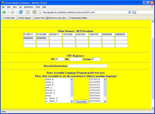
The program itself is in main memory (at the top) and occupies the first seven spaces in memory. Note that it is binary, which is a requirement for all modern computers. The next three spaces (all with 00000000) will hold the data as it is read in and processed. Thus, from all appearances, the VSC-32 is a von Neumann computer because the program and its data will share the same memory (and will all be binary in form).
Although you need not
worry about this now, some of you may be curious as to what’s going on at the
bottom of the screenshot.
Here goes…
At the bottom left is an area where you can type in a program. Can you see that 9 lines are visible?
The first 7 lines look like instructions and the last 2 lines like data, don’t they?
In fact, this is the program of Figure 1.7 on page 7 of your textbook, except that it is written in a language
designed especially for the VSC-32 computer.
Once the program on the left is typed in, the Assemble button is clicked, causing everything on the left to be translated into binary.
The result appears in the area on the right. Notice that the same number of lines appears on the right, but in binary.
Thus, each line on the left gets translated into some pattern of 8 bits (0’s and 1’s) seen on the right.
These patterns are then loaded into memory at the top, at which time you can actually run the program.
If you understood very little of what I wrote after the screenshot,
don’t worry now. We’ll understand it all
later in the semester.
Computers: Their History and Their Limitations
Finally, there is a very quick treatment of the history of computing on pages 9-10 of your textbook. It’s amazing what progress has occurred in the last few decades, and, in particular, the last twenty years. More detail, in the form of a computing history timeline can be found at this site.
It is tempting to believe that computers are all powerful, given what we see them do on a daily basis. But remember that they can only do what we can program them to do. And, sometimes, even if we have a program that will eventually solve the problem, we’ll find that it cannot solve it in any feasible amount of time. One example of this is the problem of factoring an integer, that is, when given a number as input, list as output all numbers that are divisors of the number. (Thus, if the input is 12, the output is 1 2 3 4 6 12).
Not even the fastest computer in the world can be expected to factor a 200-digit number in your lifetime, even if it started this very second. That is because no one has yet thought of an efficient algorithm (a step-by-step method) for factoring. In computer science, it is said then that factoring is hard. Yet, if you care about national security and secure communications, this is not a bad thing, as we shall see when we study some cryptography at the very end of the course.
Two Different
Algorithms for finding the Greatest Common Divisor of Two Numbers
To close this week out, let’s think of how we might think about how to solve the problem of finding the greatest common divisor (the GCD) of two numbers. For example, the GCD of 12 and 18 is 6. An obvious (naïve) algorithm is the following:
ALGORITHM A for GCD:
1. List all divisors of the first input.
2. List all divisors of the second input.
3. Make a third list consisting of all numbers that occur in both lists.
4. Find the greatest (sounds familiar!) of the numbers in the third list and report that as output.
Try to follow the steps of this algorithm as you play with this site.
Try numbers like 500 and 140 and then others that come to mind.
Do you think this is an efficient algorithm for finding the GCD? Why or why not?
Do you think we can find the GCD of two 200-digit numbers using this algorithm? Why or why not?
Remember that factoring is hard.
Algorithm B for GCD:
Now let’s try a new approach. Actually, a very old approach since it was invented about 2300 years ago by the ancient Greek mathematician Euclid.
I’m about to send you to a site I developed that allows you to track a program as it steps through Euclid’s GCD algorithm. When you visit the site, please enter two numbers at the top (e.g. 500 and 140), then slowly and repeatedly click the Step button while tracking the values of I, J, and R.
OK, I’ll let you try it now:
Euclid's GCD algorithm.
The remarkable thing about this algorithm is that it does not factor either of its input values!
It is, in fact, possible to find the GCD of two 200-digit numbers using this algorithm, even though factoring either of the two numbers is not feasible!
I will convince you all of this in class!
Conclusions: Euclid was a great computer scientist, and, oh yeah, factoring is hard…