In class, we talked about using Euler's method to approximate the solution of a differential equation numerically.
Suppose that we have a differential equation \[\frac{dy}{dx} = F(x,y)\] where \(F(x,y)\) is some function that involves x and/or y. You will need to choose a step size \(\Delta x\). You can start with \(\Delta x = 0.1\) and then adjust from there.
Euler's method is recursive, that is, it uses what you know about your current x and y-values to find the next x and y-values. Here are the formulas for how to do this:
\[x_{n+1} = x_n+\Delta x\] \[y_{n+1} = y_n+F(x_n,y_n)\Delta x\]
Suppose we want to create a numerical approximation for the explosion equation \[\frac{dy}{dx} = y^2\] with initial condition \(y(0)=1\).
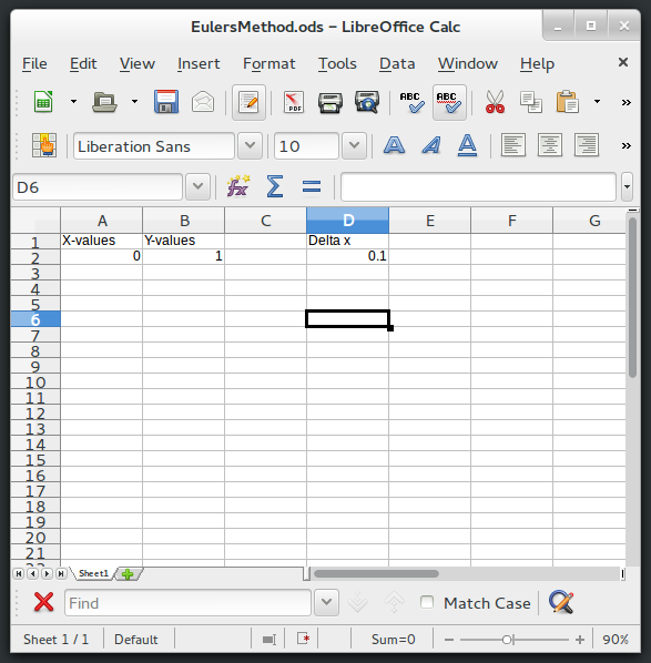
First enter your initial conditions into a spreadsheet, and also make a note of the step size \(\Delta x\).
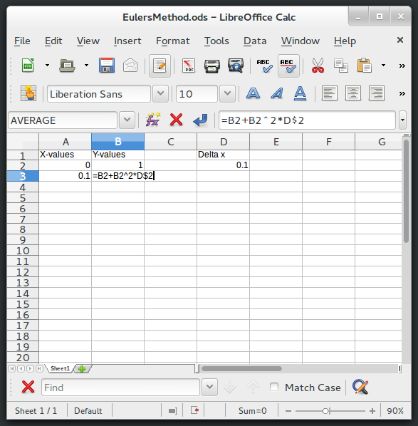
Now enter the formulas in the cells directly below the initial conditions. The next x-value should be entered into cell A3 as: =A2+D$2. The next y-value goes in B3, and it would be =B2+B2^2*D$2. The dollar sign makes sure that when we drag these cells down, the formulas always use cell D2 for \(\Delta x\) and not the cells below D2.
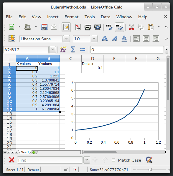
Now you can copy and paste the formulas for x and y into the cells below to update the spreadsheet. Here's how that looks. If you highlight cells A3 and B3, you can hold down the little black square in the bottom right corner to do this.

Notice, that these results aren't very accurate (after all, the explosion equation with these initial conditions has a vertical asymptote at \(x=1\)!). To improve the accuracy, try making \(\Delta x\) smaller. You can also insert a graph by clicking on the insert tab and finding the option to insert a scatter plot (lines only).