Bootstrap Method Example

The file HighPeaks.csv contains data about the 46 "high peaks" in the Adirondaks of upstate New York. A goal for hikers in the region is to scale all 46 peaks. The data in the file gives the elevation (in feet), round trip distance (in miles), difficulty (scale of 1 to 7, with 7 being the most difficult), and expected trip time (hours) for each of the 46 hikes.

myData = read.csv("HighPeaks.csv")
head(myData)

	Peak	Elevation	Difficulty	Ascent	Length	Time
1	Mt. Marcy	5344	5	3166	14.8	10
2	Algonquin Peak	5114	5	2936	9.6	9
3	Mt. Haystack	4960	7	3570	17.8	12
4	Mt. Skylight	4926	7	4265	17.9	15
5	Whiteface Mtn.	4867	4	2535	10.4	8.5
6	Dix Mtn.	4857	5	2800	13.2	10

myLM = lm(Length~Time,myData)
plot(Length~Time,myData)
abline(myLM)

The regression line above shows how the length of a hike can be predicted from the time it takes to complete. The slope has units miles per hour, so it measures the average speed of hikers on these trails. We can use the bootstrap method to make a confidence interval for this average speed.

bootstrapDistribution = c()
for (i in 1:5000) {
    bootstrapSample = myData[sample(1:nrow(myData),nrow(myData),replace=TRUE),]
    bootstrapStatistic = summary(lm(Length~Time,bootstrapSample))$coefficients["Time","Estimate"]
    bootstrapDistribution = c(bootstrapDistribution,bootstrapStatistic)
}
hist(bootstrapDistribution,col='gray')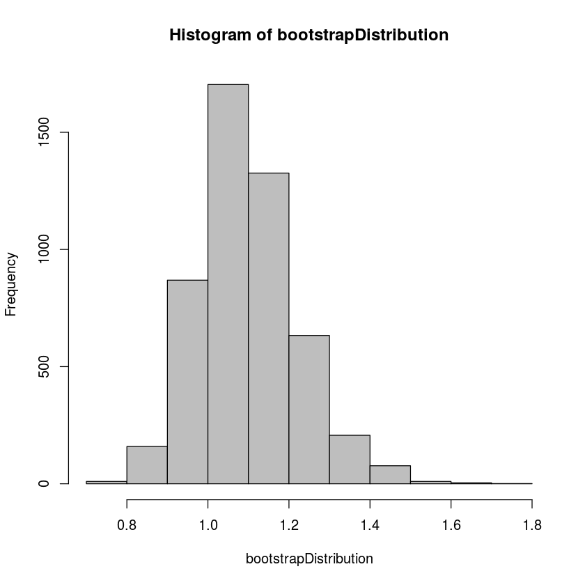

quantile(bootstrapDistribution,0.025)
quantile(bootstrapDistribution,0.975)

2.5%: 0.887998602994118

97.5%: 1.37734361978935

These quantiles are the upper and lower bound for a 95% confidence interval for the slope of the regression line. That is, based on the bootstrap distribution, we can be 95% certain that the slope of the regression line is between 0.888 miles per hour and 1.377 miles per hour.

We could just as easily construct a bootstrap distribution for any other regression statistic. Here is one for the correlation coefficient.

bootstrapDistribution = c()
for (i in 1:5000) {
    bootstrapSample = myData[sample(1:nrow(myData),nrow(myData),replace=TRUE),]
    bootstrapStatistic = cor(bootstrapSample$Length,bootstrapSample$Time)
    bootstrapDistribution = c(bootstrapDistribution,bootstrapStatistic)
}
hist(bootstrapDistribution,col='gray')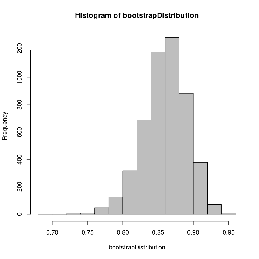

quantile(bootstrapDistribution,0.025)
quantile(bootstrapDistribution,0.975)

2.5%: 0.792745667787344

97.5%: 0.915294566358632

So we can be 95% percent certain that the correlation coefficient is between 0.793 and 0.915.

Note: there are other ways to make bootstrap confidence intervals, but using the region between the quantiles is probably the simplest.