From OpenIntro Stats.
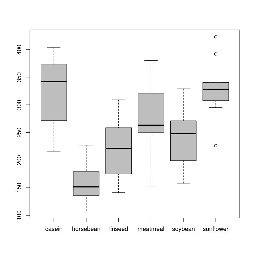
Chicken farming is a multi-billion dollar industry, and any methods that increase the growth rate of young chicks can reduce consumer costs while increasing company profits, possibly by millions of dollars. An experiment was conducted to measure and compare the effectiveness of various feed supplements on the growth rate of chickens. Newly hatched chicks were randomly allocated into six groups, and each group was given a different feed supplement. Below are some summary statistics from this data set along with box plots showing the distribution of weights by feed type.
chickenData = read.csv('chickwts.csv')
dim(chickenData)
head(chickenData)| weight | feed | |
|---|---|---|
| 1 | 179 | horsebean |
| 2 | 160 | horsebean |
| 3 | 136 | horsebean |
| 4 | 227 | horsebean |
| 5 | 217 | horsebean |
| 6 | 168 | horsebean |
The command unique() can list the distinct categories of feed the chickens are fed.
unique(chickenData$feed)boxplot(weight~feed,data=chickenData,col='gray')The boxplots are pretty different. Casein feed looks much better than horsebean for example. But the sample sizes in each group are very small, so it is not obvious that the differences will be statistically significant. Below is an example of how to do ANOVA with R.
results=aov(weight~feed,data=chickenData)
summary(results)
Df Sum Sq Mean Sq F value Pr(>F)
feed 5 231129 46226 15.37 5.94e-10 ***
Residuals 65 195556 3009
---
Signif. codes: 0 ‘***’ 0.001 ‘**’ 0.01 ‘*’ 0.05 ‘.’ 0.1 ‘ ’ 1Based on the F-value and its p-value, we should be able to safely reject the null hypothesis and conclude that there are differences in the mean weight of chickens that are feed different chicken feeds. Before we do that, let's double check that data in each group is roughly normal. Because the groups are so small, a qq-plot is probably a better choice than a histogram.
par(mfrow=c(3,2))
qqnorm(subset(chickenData,feed=='casein')$weight)
qqnorm(subset(chickenData,feed=='horsebean')$weight)
qqnorm(subset(chickenData,feed=='linseed')$weight)
qqnorm(subset(chickenData,feed=='meatmeal')$weight)
qqnorm(subset(chickenData,feed=='soybean')$weight)
qqnorm(subset(chickenData,feed=='sunflower')$weight)
These normal quantile plots are reasonably close to straight lines, so the normality assumption is probably okay. We also need to double check that the constant variance assumption isn't way off. The rule of thumb from the book was to make sure that none of the sample standard devitions are separated by a factor greater than 2. Here is one way to quickly calculate the sample standard deviation for each group:
aggregate(weight~feed,data=chickenData,FUN=sd)| feed | weight | |
|---|---|---|
| 1 | casein | 64.43384 |
| 2 | horsebean | 38.62584 |
| 3 | linseed | 52.2357 |
| 4 | meatmeal | 64.90062 |
| 5 | soybean | 54.12907 |
| 6 | sunflower | 48.83638 |
Since the ratio of the largest std. dev. (64.9) to the smallest (38.6) is less than 2, we are probably safe assuming that the data has a constant standard deviation. We also don't need to worry about the independence assumption since this was a random sample of chickens. Therefore our conclusion that the difference are significant is almost certainly valid.
R can quickly compute the t-value and corresponding p-value for each pairwise comparison between two groups. Here are the sample means for the groups:
aggregate(weight~feed,data=chickenData,FUN=mean)| feed | weight | |
|---|---|---|
| 1 | casein | 323.5833 |
| 2 | horsebean | 160.2 |
| 3 | linseed | 218.75 |
| 4 | meatmeal | 276.9091 |
| 5 | soybean | 246.4286 |
| 6 | sunflower | 328.9167 |
pairwise.t.test(chickenData$weight,chickenData$feed,p.adj='bonferroni') Pairwise comparisons using t tests with pooled SD
data: chickenData$weight and chickenData$feed
casein horsebean linseed meatmeal soybean
horsebean 3.1e-08 - - - -
linseed 0.00022 0.22833 - - -
meatmeal 0.68350 0.00011 0.20218 - -
soybean 0.00998 0.00487 1.00000 1.00000 -
sunflower 1.00000 1.2e-08 9.3e-05 0.39653 0.00447
P value adjustment method: bonferroni Notice the argument p.adj, which is the method for adjusting significance levels to avoid type I errors. In this case, there are 15 pairwise comparison, so R has increased all of the p-values by a factor of 15 to compensate. Notice that multiplying the p-values by 15 is pretty much the same as dividing the \(\alpha\) by 15. This way, however, if a p-value in the table above looks significant (i.e., below 0.05), then we can safely conclude that it is statistically significant.
It is also possible to construct confidence intervals for each difference above. The most common technique is known as Tukey's Honest Significant Differences, and the command is TukeyHSD(), as shown below:
TukeyHSD(results,conf.level=0.95) Tukey multiple comparisons of means
95% family-wise confidence level
Fit: aov(formula = weight ~ feed, data = chickenData)
$feed
diff lwr upr p adj
horsebean-casein -163.383333 -232.346876 -94.41979 0.0000000
linseed-casein -104.833333 -170.587491 -39.07918 0.0002100
meatmeal-casein -46.674242 -113.906207 20.55772 0.3324584
soybean-casein -77.154762 -140.517054 -13.79247 0.0083653
sunflower-casein 5.333333 -60.420825 71.08749 0.9998902
linseed-horsebean 58.550000 -10.413543 127.51354 0.1413329
meatmeal-horsebean 116.709091 46.335105 187.08308 0.0001062
soybean-horsebean 86.228571 19.541684 152.91546 0.0042167
sunflower-horsebean 168.716667 99.753124 237.68021 0.0000000
meatmeal-linseed 58.159091 -9.072873 125.39106 0.1276965
soybean-linseed 27.678571 -35.683721 91.04086 0.7932853
sunflower-linseed 110.166667 44.412509 175.92082 0.0000884
soybean-meatmeal -30.480519 -95.375109 34.41407 0.7391356
sunflower-meatmeal 52.007576 -15.224388 119.23954 0.2206962
sunflower-soybean 82.488095 19.125803 145.85039 0.0038845From this table, we can see from the bottom row that the difference between the average weights of chickens fed sunflower feed versus soybean feed will be between 19.1 ounces and 145.8 ounces (with 95%) confidence. Notice that the adjusted p-values are little lower than the ones using the Bonferroni condition. The Tukey method is a little more complicated, and it is a little less conservative.