Below is data from a sample of couples registering for marriage licenses. The data includes both the husband and the wife's ages. This is matched pairs data, so the only appropriate permutation would be to swap the ages of husbands with their wives, effectively swapping the signs of the differences. This is easy to do with R.

marriageData=read.csv("marriageAges.csv")
differences = marriageData$Husband - marriageData$Wife
t.test(differences)

    One Sample t-test

data:  differences
t = 1.9088, df = 23, p-value = 0.06884
alternative hypothesis: true mean is not equal to 0
95 percent confidence interval:
 -0.1570288  3.9070288
sample estimates:
mean of x 
    1.875 

tvalues = c()
for (i in 1:10000) {
    resampleDifferences = differences*sample(c(-1,1),length(differences),replace=TRUE)
    tvalues = c(tvalues,t.test(resampleDifferences)$statistic)
}
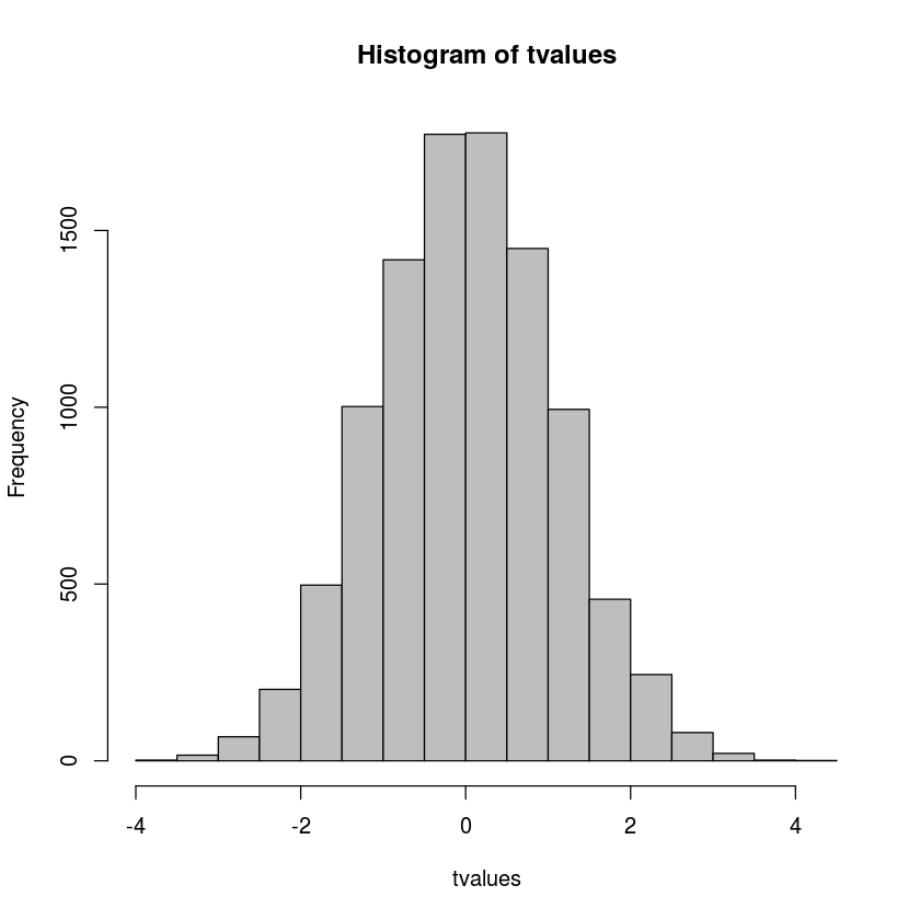
hist(tvalues,col='gray')

(sum(tvalues>1.9088)+sum(tvalues < -1.9088))/10000

0.0636

The two-sided permutation test p-value above is very close to the classical p-value, which isn't really that surprising. In this case it suggests that the evidence isn't quite strong enough to conclude that there is a difference in the average ages between husbands and their wives.

Bootstrap Confidence Interval

We can also make a bootstrap distribution for the differences.

meanDistribution = c()
for (i in 1:1000) {
    meanDistribution = c(meanDistribution,mean(sample(differences,replace=TRUE)))
}
hist(meanDistribution,col='gray')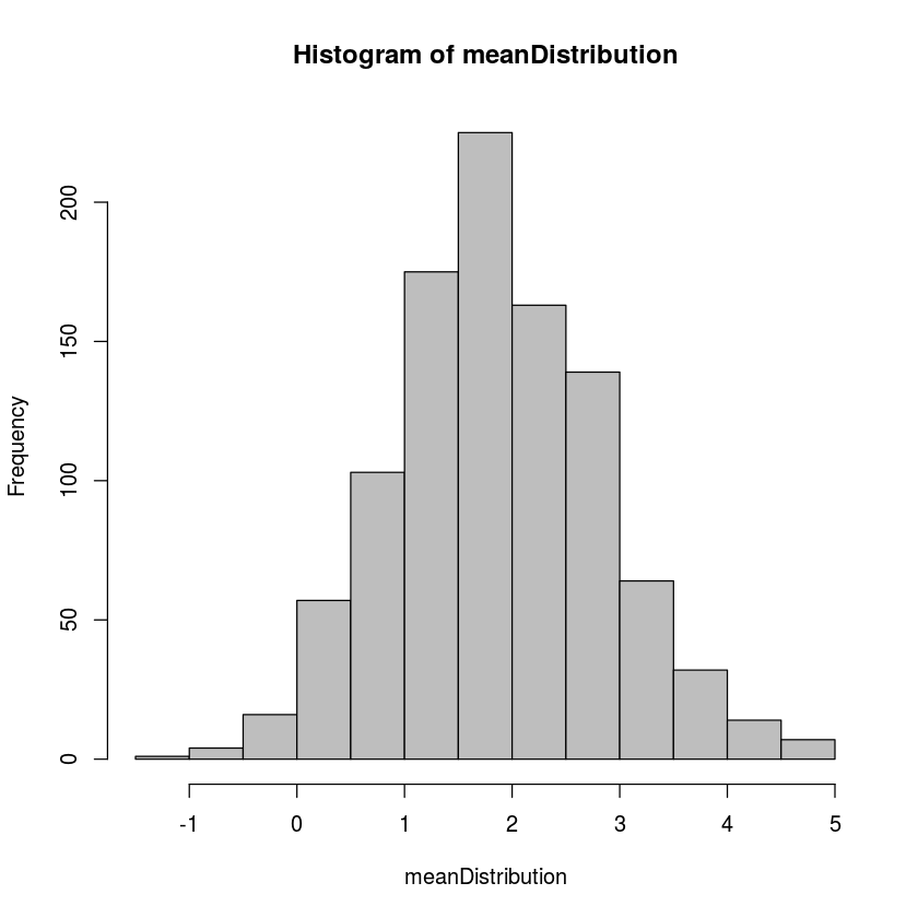

quantile(meanDistribution,0.025)
quantile(meanDistribution,0.975)

2.5%: 0.0822916666666667

97.5%: 3.91666666666667

This bootstrap confidence interval says we can be 95% sure that the average age difference (husband's age minus wife's age) is between 0.0823 and 3.9167 years. Unlike the permutation method, this suggests that the differences are statistically significant, but it is probably best to be cautious when two valid tests give different answers.