In the 2014 General Social Survey, respondents were asked questions about many topics, including their religion and income. Below is a two-way analysis of variance for differences in income due to two factors: region (Northeast, South, Midwest, or West) and religion (Catholic, Protestant, or Other).
myData = read.csv('RegionReligionIncome2.csv')head(myData)
dim(myData)| Household_Income | Region | Religion | Income_Number | |
|---|---|---|---|---|
| 1 | 75000 to 89999 | Northeast | Catholic | 82500 |
| 2 | 150000 or over | Northeast | Catholic | 250000 |
| 3 | 40000 to 49999 | Northeast | Protestant | 45000 |
| 4 | 150000 or over | Northeast | Catholic | 250000 |
| 5 | Refused | Northeast | Catholic | NA |
| 6 | 150000 or over | Northeast | Protestant | 250000 |
Once again, this data has a lot of NA entries. So we will use the na.omit() command to clean things up.
myData=na.omit(myData)
head(myData)
dim(myData)| Household_Income | Region | Religion | Income_Number | |
|---|---|---|---|---|
| 1 | 75000 to 89999 | Northeast | Catholic | 82500 |
| 2 | 150000 or over | Northeast | Catholic | 250000 |
| 3 | 40000 to 49999 | Northeast | Protestant | 45000 |
| 4 | 150000 or over | Northeast | Catholic | 250000 |
| 6 | 150000 or over | Northeast | Protestant | 250000 |
| 8 | 75000 to 89999 | Northeast | Catholic | 82500 |
par(mfrow=c(2,2))
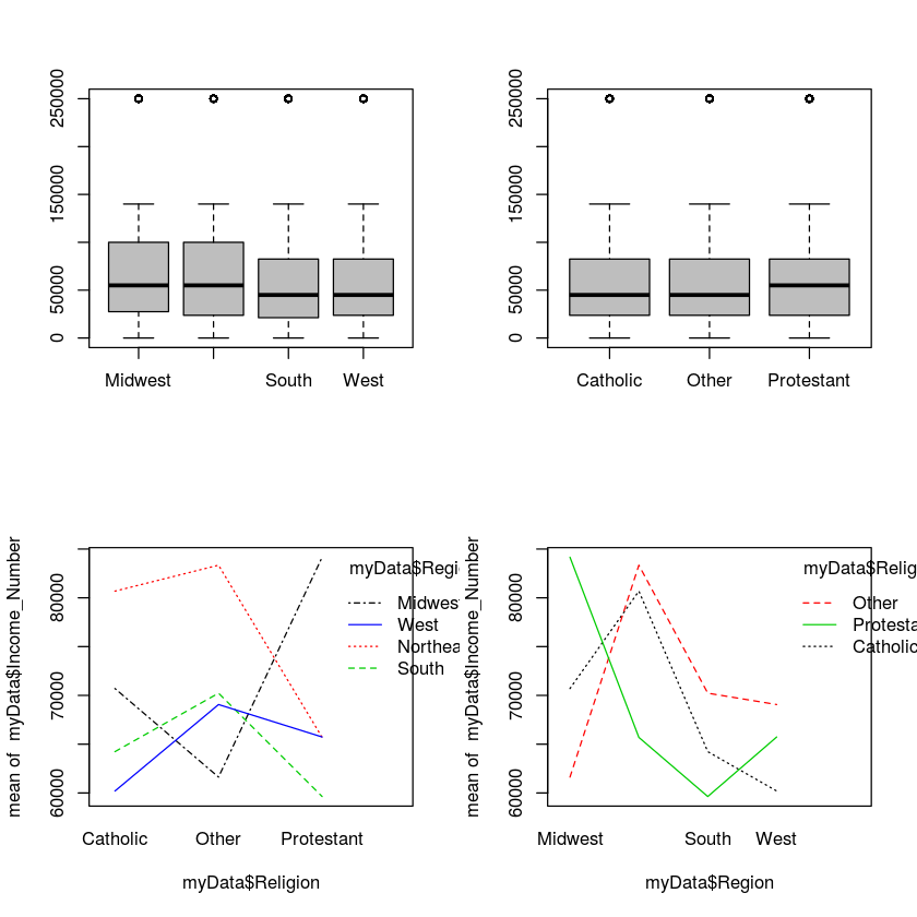
boxplot(Income_Number~Region,data=myData,col='gray')
boxplot(Income_Number~Religion,data=myData,col='gray')
interaction.plot(myData$Religion,myData$Region,myData$Income_Number,col=c(1,2,3,4))
interaction.plot(myData$Region,myData$Religion,myData$Income_Number,col=c(1,2,3,4))From this interaction plot, it looks like there is an interaction between region and religion. For example, Catholics make more money than Protestants in the Northeast, but they make less money in the South and West.
table(myData$Region,myData$Religion) Catholic Other Protestant
Midwest 120 155 249
Northeast 134 145 112
South 173 178 496
West 121 252 179The table command can be used to find the counts for each cell. From this we can see that most of the cells are about the same size, although there are some, like Protestants in the South that are much larger.
myAOV = aov(Income_Number ~ Region * Religion, data = myData)
summary(myAOV)
model.tables(myAOV,'means')
#?model.tables
Df Sum Sq Mean Sq F value Pr(>F)
Region 3 7.990e+10 2.663e+10 6.116 0.000385 ***
Religion 2 1.987e+09 9.935e+08 0.228 0.796019
Region:Religion 6 9.215e+10 1.536e+10 3.527 0.001772 **
Residuals 2302 1.002e+13 4.355e+09
---
Signif. codes: 0 ‘***’ 0.001 ‘**’ 0.01 ‘*’ 0.05 ‘.’ 0.1 ‘ ’ 1
Tables of means
Grand mean
68666.92
Region
Midwest Northeast South West
74413 77377 62802 66042
rep 524 391 847 552
Religion
Catholic Other Protestant
67826 69992 68178
rep 548 730 1036
Region:Religion
Religion
Region Catholic Other Protestant
Midwest 70702 61629 84160
rep 120 155 249
Northeast 80685 83343 65694
rep 134 145 112
South 64236 70229 59637
rep 173 178 496
West 60202 69063 65736
rep 121 252 179 We need to check that the residuals obey the following assumptions.
The first assumption will automatically if the data for each cell comes from a SRS of the whole population (assuming that the population is very large). We can be pretty sure that this is basically correct, since the general social survey is a very reputable survey run by people who know a lot about statistics.
To check the second assumption, we can use the tapply() function to find the standard deviation for each subgroup in our study:
tapply(myData$Income_Number,list(myData$Region,myData$Religion),sd)| Catholic | Other | Protestant | |
|---|---|---|---|
| Midwest | 60319.39 | 59621.43 | 76522.09 |
| Northeast | 73418.60 | 77886.68 | 68138.84 |
| South | 70879.39 | 69892.39 | 56320.61 |
| West | 56246.46 | 70059.87 | 56845.68 |
The gap between the largest and smallest sample standard deviation much less than a factor of 2, so assumption #2 is probably okay. Let us turn to assumption #3.
qqnorm(resid(myAOV))
par(mfrow=c(4,3))
qqnorm(subset(myData,Region=='Midwest' & Religion=='Catholic')$Income_Number)
qqnorm(subset(myData,Region=='Midwest' & Religion=='Other')$Income_Number)
qqnorm(subset(myData,Region=='Midwest' & Religion=='Protestant')$Income_Number)
qqnorm(subset(myData,Region=='Northeast' & Religion=='Catholic')$Income_Number)
qqnorm(subset(myData,Region=='Northeast' & Religion=='Other')$Income_Number)
qqnorm(subset(myData,Region=='Northeast' & Religion=='Protestant')$Income_Number)
qqnorm(subset(myData,Region=='South' & Religion=='Catholic')$Income_Number)
qqnorm(subset(myData,Region=='South' & Religion=='Other')$Income_Number)
qqnorm(subset(myData,Region=='South' & Religion=='Protestant')$Income_Number)
qqnorm(subset(myData,Region=='West' & Religion=='Catholic')$Income_Number)
qqnorm(subset(myData,Region=='West' & Religion=='Other')$Income_Number)
qqnorm(subset(myData,Region=='West' & Religion=='Protestant')$Income_Number)
par(mfrow=c(4,3))
hist(subset(myData,Region=='Midwest' & Religion=='Catholic')$Income_Number)
hist(subset(myData,Region=='Midwest' & Religion=='Other')$Income_Number)
hist(subset(myData,Region=='Midwest' & Religion=='Protestant')$Income_Number)
hist(subset(myData,Region=='Northeast' & Religion=='Catholic')$Income_Number)
hist(subset(myData,Region=='Northeast' & Religion=='Other')$Income_Number)
hist(subset(myData,Region=='Northeast' & Religion=='Protestant')$Income_Number)
hist(subset(myData,Region=='South' & Religion=='Catholic')$Income_Number)
hist(subset(myData,Region=='South' & Religion=='Other')$Income_Number)
hist(subset(myData,Region=='South' & Religion=='Protestant')$Income_Number)
hist(subset(myData,Region=='West' & Religion=='Catholic')$Income_Number)
hist(subset(myData,Region=='West' & Religion=='Other')$Income_Number)
hist(subset(myData,Region=='West' & Religion=='Protestant')$Income_Number)
The data in each cell is clearly not normal, but that really won't be a problem. Because the sample sizes in each cell are so large (over 100), the means for each cell will definitely have a normal distribution due to the central limit theorem. Therefore using ANOVA in this situation is probably fine.
We can use the TukeyHSD() command to get confidence intervals for all of the pairwise differences in our model. There are a lot! Also, most of the differences are not statistically significant.
TukeyHSD(myAOV,conf.level=0.95) Tukey multiple comparisons of means
95% family-wise confidence level
Fit: aov(formula = Income_Number ~ Region * Religion, data = myData)
$Region
diff lwr upr p adj
Northeast-Midwest 2963.431 -8373.991 14300.8518 0.9076886
South-Midwest -11611.220 -21040.296 -2182.1439 0.0085133
West-Midwest -8371.048 -18718.388 1976.2914 0.1599661
South-Northeast -14574.650 -24947.259 -4202.0417 0.0017606
West-Northeast -11334.479 -22548.353 -120.6045 0.0464494
West-South 3240.172 -6039.987 12520.3295 0.8060734
$Religion
diff lwr upr p adj
Other-Catholic 2165.2074 -6581.981 10912.395 0.8305636
Protestant-Catholic 351.7939 -7822.724 8526.312 0.9943998
Protestant-Other -1813.4135 -9291.815 5664.988 0.8368036
$`Region:Religion`
diff lwr upr
Northeast:Catholic-Midwest:Catholic 9982.61816 -17149.17128 37114.40760
South:Catholic-Midwest:Catholic -6466.53420 -32112.83534 19179.76694
West:Catholic-Midwest:Catholic -10499.60399 -38311.44994 17312.24195
Midwest:Other-Midwest:Catholic -9073.05108 -35322.15466 17176.05251
Northeast:Other-Midwest:Catholic 12641.02011 -14000.12663 39282.16686
South:Other-Midwest:Catholic -473.15075 -25971.50261 25025.20111
West:Other-Midwest:Catholic -1638.59127 -25581.95585 22304.77331
Midwest:Protestant-Midwest:Catholic 13457.55522 -10532.29235 37447.40279
Northeast:Protestant-Midwest:Catholic -5007.88690 -33370.67760 23354.90379
South:Protestant-Midwest:Catholic -11065.49059 -33027.06629 10896.08511
West:Protestant-Midwest:Catholic -4966.04981 -30435.70454 20503.60491
South:Catholic-Northeast:Catholic -16449.15236 -41291.82628 8393.52156
West:Catholic-Northeast:Catholic -20482.22215 -47554.79979 6590.35548
Midwest:Other-Northeast:Catholic -19055.66923 -44520.17638 6408.83791
Northeast:Other-Northeast:Catholic 2658.40196 -23210.04185 28526.84576
South:Other-Northeast:Catholic -10455.76891 -35145.67844 14234.14062
West:Other-Northeast:Catholic -11621.20943 -34701.72919 11459.31033
Midwest:Protestant-Northeast:Catholic 3474.93706 -19653.79986 26603.67398
Northeast:Protestant-Northeast:Catholic -14990.50506 -42628.76805 12647.75792
South:Protestant-Northeast:Catholic -21048.10875 -42065.63697 -30.58053
West:Protestant-Northeast:Catholic -14948.66797 -39608.93960 9711.60366
West:Catholic-South:Catholic -4033.06979 -29616.72129 21550.58170
Midwest:Other-South:Catholic -2606.51687 -26482.02500 21268.99125
Northeast:Other-South:Catholic 19107.55432 -5198.31224 43413.42087
South:Other-South:Catholic 5993.38345 -17054.18468 29040.95158
West:Other-South:Catholic 4827.94293 -16486.58630 26142.47216
Midwest:Protestant-South:Catholic 19924.08942 -1442.64256 41290.82140
Northeast:Protestant-South:Catholic 1458.64730 -24722.87949 27640.17408
South:Protestant-South:Catholic -4598.95639 -23660.31144 14462.39866
West:Protestant-South:Catholic 1500.48439 -21515.33107 24516.29984
Midwest:Other-West:Catholic 1426.55292 -24761.34315 27614.44899
Northeast:Other-West:Catholic 23140.62411 -3440.21789 49721.46611
South:Other-West:Catholic 10026.45325 -15408.88456 35461.79105
West:Other-West:Catholic 8861.01272 -15015.23423 32737.25968
Midwest:Protestant-West:Catholic 23957.15922 34.29886 47880.01957
Northeast:Protestant-West:Catholic 5491.71709 -22814.43696 33797.87114
South:Protestant-West:Catholic -565.88660 -22454.26865 21322.49546
West:Protestant-West:Catholic 5533.55418 -19873.01531 30940.12367
Northeast:Other-Midwest:Other 21714.07119 -3227.01591 46655.15829
South:Other-Midwest:Other 8599.90033 -15116.61446 32316.41511
West:Other-Midwest:Other 7434.45981 -14601.68853 29470.60814
Midwest:Protestant-Midwest:Other 22530.60630 443.96073 44617.25186
Northeast:Protestant-Midwest:Other 4065.16417 -22707.11668 30837.44502
South:Protestant-Midwest:Other -1992.43952 -21857.43217 17872.55314
West:Protestant-Midwest:Other 4107.00126 -19578.65764 27792.66017
South:Other-Northeast:Other -13114.17086 -37263.87758 11035.53585
West:Other-Northeast:Other -14279.61138 -36781.32452 8222.10175
Midwest:Protestant-Northeast:Other 816.53511 -21734.63278 23367.70299
Northeast:Protestant-Northeast:Other -17648.90702 -44805.67933 9507.86529
South:Protestant-Northeast:Other -23706.51071 -44086.72646 -3326.29495
West:Protestant-Northeast:Other -17607.06993 -41726.47495 6512.33509
West:Other-South:Other -1165.44052 -22301.72074 19970.83970
Midwest:Protestant-South:Other 13930.70597 -7258.21615 35119.62809
Northeast:Protestant-South:Other -4534.73616 -30571.35518 21501.88287
South:Protestant-South:Other -10592.33984 -29454.16483 8269.48514
West:Protestant-South:Other -4492.89906 -27343.74032 18357.94219
Midwest:Protestant-West:Other 15096.14649 -4193.46679 34385.75977
Northeast:Protestant-West:Other -3369.29563 -27885.09238 21146.50111
South:Protestant-West:Other -9426.89932 -26126.81553 7273.01689
West:Protestant-West:Other -3327.45854 -24429.11028 17774.19319
Northeast:Protestant-Midwest:Protestant -18465.44213 -43026.63853 6095.75428
South:Protestant-Midwest:Protestant -24523.04581 -41289.53860 -7756.55302
West:Protestant-Midwest:Protestant -18423.60503 -39577.98484 2730.77477
South:Protestant-Northeast:Protestant -6057.60369 -28641.89889 16526.69152
West:Protestant-Northeast:Protestant 41.83709 -25966.67871 26050.35290
West:Protestant-South:Protestant 6099.44078 -12723.57189 24922.45345
p adj
Northeast:Catholic-Midwest:Catholic 0.9887616
South:Catholic-Midwest:Catholic 0.9996202
West:Catholic-Midwest:Catholic 0.9861544
Midwest:Other-Midwest:Catholic 0.9933194
Northeast:Other-Midwest:Catholic 0.9255492
South:Other-Midwest:Catholic 1.0000000
West:Other-Midwest:Catholic 1.0000000
Midwest:Protestant-Midwest:Catholic 0.7984972
Northeast:Protestant-Midwest:Catholic 0.9999892
South:Protestant-Midwest:Catholic 0.8908251
West:Protestant-Midwest:Catholic 0.9999702
South:Catholic-Northeast:Catholic 0.5746521
West:Catholic-Northeast:Catholic 0.3562458
Midwest:Other-Northeast:Catholic 0.3739089
Northeast:Other-Northeast:Catholic 1.0000000
South:Other-Northeast:Catholic 0.9664043
West:Other-Northeast:Catholic 0.8912900
Midwest:Protestant-Northeast:Catholic 0.9999980
Northeast:Protestant-Northeast:Catholic 0.8320198
South:Protestant-Northeast:Catholic 0.0492740
West:Protestant-Northeast:Catholic 0.7051412
West:Catholic-South:Catholic 0.9999967
Midwest:Other-South:Catholic 0.9999999
Northeast:Other-South:Catholic 0.2964306
South:Other-South:Catholic 0.9994899
West:Other-South:Catholic 0.9998663
Midwest:Protestant-South:Catholic 0.0951096
Northeast:Protestant-South:Catholic 1.0000000
South:Protestant-South:Catholic 0.9997519
West:Protestant-South:Catholic 1.0000000
Midwest:Other-West:Catholic 1.0000000
Northeast:Other-West:Catholic 0.1608574
South:Other-West:Catholic 0.9805024
West:Other-West:Catholic 0.9879418
Midwest:Protestant-West:Catholic 0.0492845
Northeast:Protestant-West:Catholic 0.9999716
South:Protestant-West:Catholic 1.0000000
West:Protestant-West:Catholic 0.9999093
Northeast:Other-Midwest:Other 0.1608072
South:Other-Midwest:Other 0.9900278
West:Other-Midwest:Other 0.9945672
Midwest:Protestant-Midwest:Other 0.0407377
Northeast:Protestant-Midwest:Other 0.9999977
South:Protestant-Midwest:Other 1.0000000
West:Protestant-Midwest:Other 0.9999910
South:Other-Northeast:Other 0.8308946
West:Other-Northeast:Other 0.6401319
Midwest:Protestant-Northeast:Other 1.0000000
Northeast:Protestant-Northeast:Other 0.6039518
South:Protestant-Northeast:Other 0.0080218
West:Protestant-Northeast:Other 0.4144931
West:Other-South:Other 1.0000000
Midwest:Protestant-South:Other 0.5858756
Northeast:Protestant-South:Other 0.9999906
South:Protestant-South:Other 0.7973502
West:Protestant-South:Other 0.9999675
Midwest:Protestant-West:Other 0.3032525
Northeast:Protestant-West:Other 0.9999992
South:Protestant-West:Other 0.7918008
West:Protestant-West:Other 0.9999967
Northeast:Protestant-Midwest:Protestant 0.3663817
South:Protestant-Midwest:Protestant 0.0001153
West:Protestant-Midwest:Protestant 0.1604259
South:Protestant-Northeast:Protestant 0.9993160
West:Protestant-Northeast:Protestant 1.0000000
West:Protestant-South:Protestant 0.9961705