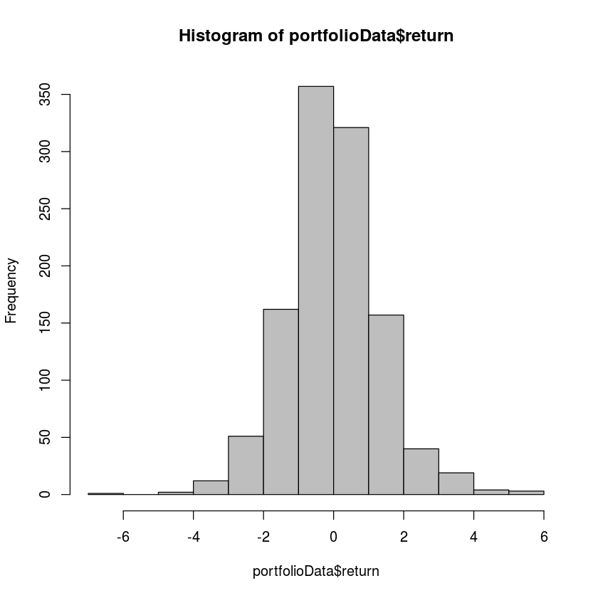
In financial theory, the standard deviation of returns on an investment is one way to measure the risk of the investment. The idea is that investment with highly variable returns are riskier than investments with returns that are always the same. The data file Portfolio.csv contains the returns (in percent) on 1129 consecutive days for one stock market portfolio. We will use bootstrapping to estimate the standard deviation (and therefore the risk) for this portfolio.
portfolioData = read.csv("Portfolio.csv")
head(portfolioData)| return | |
|---|---|
| 1 | 0.229 |
| 2 | 0.936 |
| 3 | -0.646 |
| 4 | -0.858 |
| 5 | -1.44 |
| 6 | 0.182 |
sd(portfolioData$return)1.3247529510227
hist(portfolioData$return,col='gray')To get the bootstrap distribution for standard deviation, we will collect 5000 bootstrap samples and compute the standard deviation for each.
sdResults = c()
for (i in 1:5000) {
    sdResults = c(sdResults,sd(sample(portfolioData$return,replace=TRUE)))
}
hist(sdResults,col='gray')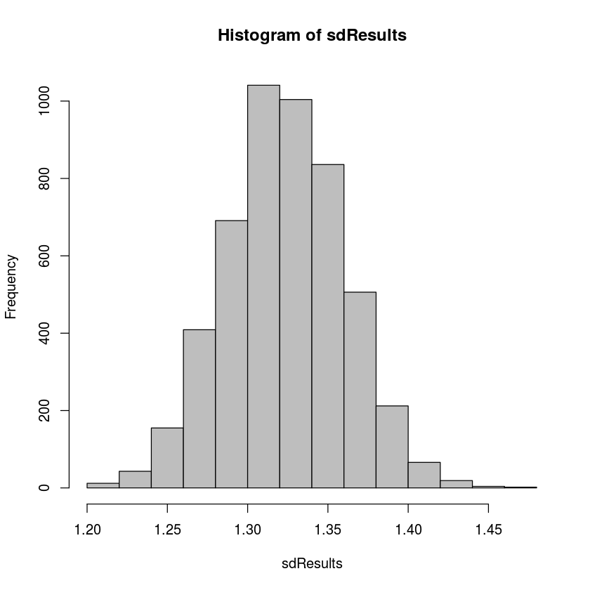
Like all bootstrap distributions, this distribution has the following important features:
The estimate for the population standard deviation is:
mean(sdResults)1.32339647051005
An estimate for the mathematical bias is:
mean(sdResults)-sd(portfolioData$return)-0.00135648051265047
This bias term above is three orders of magnitude smaller than the estimate for the parameter, so the sample standard deviation appears to be an unbiased estimator for the population parameter.
qqnorm(sdResults)
sd(sdResults)0.0373263086654002
mean(sdResults)-1.962*sd(sdResults)
mean(sdResults)+1.962*sd(sdResults)
1.24987507318962
1.39634350839265
quantile(sdResults,0.025)
quantile(sdResults,0.975)
2.5%: 1.25104406408997
97.5%: 1.39736414865592
As you can see, the t-distribution based confidence interval is very similar to the quantile based one.