Theory of Computing Notes

Computer Science 461 - Fall 2023

• Class Notes
• Schedule & Syllabus
• Software & Handouts

• 1
• 2
• 3
• 4
• 5
• 6
• 7
• 8
• 9
• 10
• 11
• 12
• 13
• 14

Week 1 Notes

Monday, Aug 21

Today we talked about proof techniques, particularly proof by induction. We looked at these two examples:

1. Prove that if a set $A$ has $n$ elements, then $A$ has $2^n$ subsets.

The second example had to do with the famous Tower’s of Hanoi puzzle( see https://youtu.be/SMleU0oeGLg).

2. Use induction to prove that it is always possible to move the disks from one peg to another by moving one disk at a time without breaking the rules.

Wednesday, Aug 23

Today we reviewed mathematical notation, including some new notation we will be using. Then we talked about encoding a finite set using binary strings. We observed that every countable set $S$ can be encoded with a 1-to-1 function from $S \rightarrow \{0,1\}^*$. We discussed specific encodings such as how to encode the integers $\mathbb{Z}$ and the rationals $\mathbb{Q}$.

• Example: ASCII characters

At the end we considered the set $\{0,1\}^\infty = \{f : f : \mathbb{N}\rightarrow \{0,1\} \}$ which you can think of as the set of all infinitely long strings of zeros and ones. We claimed, but did not have time to prove that there is no 1-to-1 encoding function $E : \{0,1\}^\infty \rightarrow \{0,1\}^*$.

Friday, Aug 25

Today we finished the proof that there is no 1-to-1 encoding function from $\{0,1\}^\infty$ to $\{0,1\}^*$.

Then we talked about Boolean circuits which are formed by AND, OR, and NOT gates.

1. Show that you can construction the function IF A THEN B ELSE C for any Boolean inputs A, B, C using AND, OR, and NOT gates.

2. Use mathematical induction to prove the following:

Theorem. Every function $f:\{0,1\}^n \rightarrow \{0,1\}$ can be represented by a Boolean circuit.

We finished by talking about how NAND gates are also universal in the sense that any function that can be constructed from AND, OR, NOT gates can also be constructed with NAND gates.

Week 2 Notes

Monday, Aug 28

Today we talked about functions $f:\{0,1\}^* \rightarrow \{0,1\}$ that cannot be computed by a computer program.

• Slides: Day 4 slides

Wednesday, Aug 30

Today we introduced finite automata. We started with three examples:

1. An automatic door at a grocery store with sensors on the front and rear. It opens if the sensor on the front is active. It won’t close until neither of the sensors are active.

2. An automatic toll both that accepts nickles, dimes, and quarters. The gate won’t open until it receives 25 cents.

3. A combination lock needs three numbers entered correctly (in order) before it will open.

With these examples we introduced state diagrams, and the definition of a deterministic finite automata (DFA).

4. Then we constructed a DFA that can compute the function $f: \{0,1\}^* \rightarrow \{0,1\}$ which returns 1 when the input string has an odd number of 1’s and 0 otherwise.

Friday, Sep 1

Today we started with these questions about DFAs:

1. For the DFA shown below:

   

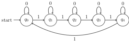
   1. What is the transition function?
   2. Describe the function $f:\{0,1\}^* \rightarrow \{0,1\}$ that this DFA computes.

2. Draw the state diagram for a DFA that computes whether a binary string contains 011.

3. Modify the DFA from the last problem so that it computer whether a binary string ends with 011.

4. How many states would a DFA need if you wanted to check whether a binary string has a 1 in the third position from the last?

After we did these examples, we defined languages which are just subsets of strings in $\Sigma^*$. Then we gave a recursive definition of regular languages and looked at some simple examples.

Week 3 Notes

Wednesday, Sep 6

Today we looked at an alternative definition of a regular language: A language $L \subseteq \Sigma^*$ is regular if and only if there is a DFA that accepts $x \in \Sigma^*$ if and only if $x \in L$. To prove that this definition is equivalent to the one we gave last week, we need to prove three things:

1. The union of two regular languages is regular.

2. The concatenation of two regular languages is regular.

3. The Kleene star of a regular language is regular.

We proved #1 in class by thinking about how to construct a new DFA $M$ that accepts $L_1 \cup L_2$ using DFAs $M_1$ and $M_2$ that accept $L_1$ and $L_2$ respectively. To prove this, we answered these questions:

1. If the machine $M$ is built by running both $M_1 = (Q_1, \Sigma, \delta_1, q_1, F_1)$ and $M_2 = (Q_2, \Sigma, \delta_2, q_2, F_2)$ simultaneously, what are the possible states of $M$?

2. What are the accepting states of $M$?

3. What are the initial states for $M$?

4. What is the transition function for $M$?

To prove that regular languages are closed under concatenation, we introduced a new idea: non-deterministic finite automata (NFAs).

We looked at this example:

We answered these questions:

5. Which states are active at each step as we read the input string 010110?

6. Does this NFA accept the string 010110?

7. Describe the set of all strings in $\{0,1\}^*$ that this NFA will accept.

Friday, September 8

Today we continued talking about NFAs. We’ve been following the textbook by Meshwari & Smid pretty closely this week, so I strongly recommend reading skimming Section 2.6 which is what we covered today.

We started with some examples of NFAs.

1. Last week we talked about how many states a DFA would need to check if a string in $\{0,1\}^*$ has a 1 in its third to last entry. We saw that a DFA needs at least 8 states for that language. But an NFA can do the job with only four states. Try to construct an example. Hint: What if the NFA “guesses” every time it sees a 1 that that might be the third to last entry. What should it’s states be from that point on?

2. Construct an NFA that accepts a string in $\{0\}^*$ iff the length of the string is a multiple of 2 or 3. Can you construct a DFA that does the same thing and with the same number of states?

After these examples, we explained two important ideas:

1. You can easily construct an NFA to check if a string is in $L_1 L_2$ when $L_1$ and $L_2$ are regular languages.

2. It is also easy to check if $x \in L^*$ when $L$ is a regular language.

For practice, see if you can construct an NFA that checks if $x \in L_1 \cup L_2$ when $L_1$ and $L_2$ are regular languages.

Week 4 Notes

Monday, September 11

Today we explained the surprising fact that any language an NFA can recognize can also be recognized by a DFA. The idea is to convert an NFA $N = (Q, \Sigma, \delta, q, F)$ into a DFA $M$ which has states that are subsets of the states of $N$, i.e., the states of $M$ are the power set $2^Q$ of the states of $N$. Then you have to make a transition function from sets of states to sets of states using the transition function $\delta$.

We looked at this example (again) to see how the idea works:

Notice that this NFA starts at state 0, and no matter what input we receive, state 0 stays active. So there is no way to reach a set of active states that does not contain state 0. So that cuts the number of elements we need to worry about in $2^Q$ by half.

We also talked about regular expressions.

Recursive Definition. A regular expression over an alphabet $\Sigma$ is a string $e$ with symbols from the extended alphabet $\Sigma \cup \{(,),*,|\}$ that has one of the following forms:

1. $e$ is a single symbol in $\Sigma$.
2. $e = e_1e_2$
3. $e = e_1|e_2$ where $e_1$ and $e_2$ are regular expressions.
4. $e = (e_1)$ where $e_1$ is a regular expression
5. $e = (e_1)*$ where $e_1$ is a regular expression

We also accept the empty set $\varnothing$ and the empty string "" as regular expressions.

Regular expressions are used to match sets of strings (i.e., languages over $\Sigma$). $e_1e_2$ matches any string that is a concatenation of a string matched by $e_1$ with a string matched by $e_2$. The regular expression $e_1|e_2$ matches anything matched by $e_1$ or $e_2$. Finally $(e_1)*$ matches any finite concatenation of strings that $e_1$ matches (including no repetitions).

1. Let $\Sigma = \{a,b,c,\ldots,z\}$. What strings does the regular expression pet(dog|cat) match?

2. What strings does the regular expression pet(dog|cat|bird)* match?

3. Find a regular expression over the alphabet $\Sigma = \{0,1\}$ that matches all strings that start with a 1, end with a 1, and have an even number of zeros between.

Wednesday, September 13

Today we mentioned the following theorem:

Theorem. A language is regular if and only if it can be represented by a regular expression.

This means that NFAs, DFAs, and RegEx’s are all equivalent to each other in terms of what they can compute. Then we looked at how to convert NFAs to RegEx’s and vice versa. We did the following examples.

1. Use the ideas from last week about how to build NFAs to find the union, concatenation, and Kleene star of languages to convert to following regular expression (ab|a)* over the alphabet Σ = {a,b} to an NFA.

Then we described an algorithm for converting NFAs to regular expressions. Note that the Maheshwwari & Smid textbook describes a different approach to convert an NFA into a regular expression in Section 2.8. We did the following example:

2. Let Σ={A,C,G,T}. Convert the following NFA to a regular expression:

We finished today by talking about some of the short-hand and quirks in regular expression libraries for some programming languages.

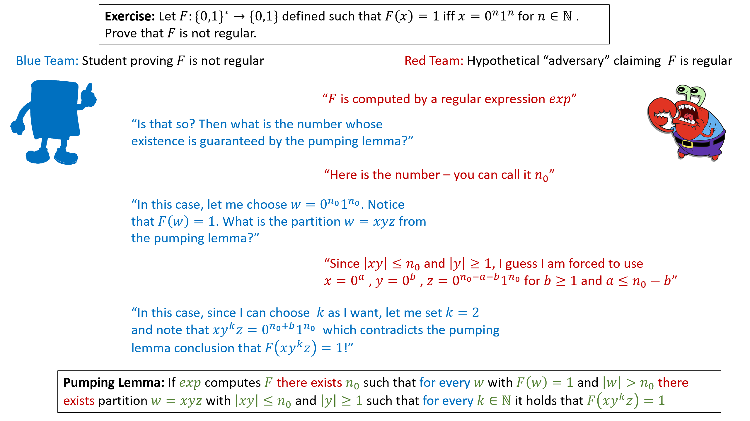
Friday, September 15

Today we talked about the pumping lemma. We used the pumping lemma to prove that the following languages over Σ = {0,1} are not regular:

1. $L = \{w : w \text{ has an equal number of 0 and 1's}\}$

2. $L = \{ww : w ∈ {0,1}^* \}$

3. $L = \{0^{n^2} : n \in \mathbb{N}\}$.

Here is a nice meme proof using the pumping lemma from Barak textbook.

Week 5 Notes

Monday, September 18

Today we looked at more examples of regular and non-regular languages.

1. $L = \{0^{n^2} : n \in \mathbb{N}\}$.

2. $L = \{w : w \text{ contains an equal number of } 01 \text{ and } 10 \text{ substrings}\}$.

Many programming languages, including Python & Javascript allow backreferences to previous groups in a regular expression. A group is a part of the regular expression inside parentheses. The special symbol \1 refers to anything matched by the first group in the regular expression. Similarly \2 refers back to anything matched by the second group, and so on. For example: the regular expression "([a-z]*) \1" would match “word word” or “dog dog”.

3. Explain why regular expressions with backreferences are not really regular expressions (at least not according to our definition).

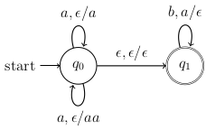
We finished with this last example. Consider the language $$F = \{a^i b^j c^k : i, j, k \ge 0 \text{ and if } i = 1 \text{ then } j = k\}.$$

4. Explain why there is a pumping number $p$ (in fact $p=1$ works) such that any string $s \in F$ can be “pumped”.

5. Despite this, explain why $F$ is not a regular language.

6. Why doesn’t that contradict the pumping lemma?

Week 6 Notes

Monday, September 25

Today we introduced context-free grammars. We started with some simple examples from Wikipedia (https://en.wikipedia.org/wiki/Context-free_grammar#Examples) to illustrate the definition.

1. We found a context free grammar that generates the (non-regular) language $L = \{a^n b^n : n \in \mathbb{N}\}$.

2. We looked at the example of a CFG and used it to identify the parts $(V,\Sigma, R, S)$ in the formal definition.

    S         →  <subject> <verb>
    <subject> →  <article> <noun>
    <article> →  a | the
    <noun>    →  boy | girl | dog
    <verb>    →  runs | jumps | swims

3. Find a context-free grammar for the language $\{w \in \{a,b\}^* : w \text{ has an equal number of } a\text{'s and } b \text{'s} \}$.

4. Describe how to generate the string (a + a) * a using the context free grammar below:

    <expr>    →  <expr> + <term> | <term>
    <term>    →  <term> * <factor> | <factor>
    <factor>  →  (<expr>) | a

We finished by looking at this example that gives the idea of how a programming language can be though of as a context-free language.

• https://en.wikipedia.org/wiki/Context-free_grammar#/media/File:C_grammar_stmt_svg.svg

Wednesday, September 27

Today, we briefly went over the first midterm exam. I talked about the grading scale and went over some of the problems .

Today we spent more time discussing context free grammars. We talked about left derivations and right derivations

We looked at this example:

$$E \rightarrow ~E+E~ | ~E*E~ | ~(E)~ | ~a~$$

1. Use this CFG to derive the string $a+a*a$. Try to use a left derivation. Then use a right derivation.

2. Show that that string actually has more than one left derivation.

A grammar is ambiguous if there are strings with more than one left derivation. If every left-derivation is unique, then the grammar is unambiguous. Note that some CFGs have unambiguous grammars, but so do not. This alternate grammar generates the same language as our first example, but is unambiguous:

    <expr>    →  <expr> + <term> | <term>
    <term>    →  <term> * <factor> | <factor>
    <factor>  →  (<expr>) | a

We looked at this ambiguous grammar.

3. Show that the sentence “the girl touches the boy with the flower” has two left derivations and those derivations correspond to two different meanings this sentence can have.
   

Friday, September 29

Today we discussed the pumping lemma for context-free languages. This is a little more complicated than the pumping lemma for regular languages. We drew some pictures of parse trees to give an intuitive explanation for why this new pumping lemma is true (see page 126 in Maheshwari & Smid). In particular, we looked at how the string a+a*a gets generated by the grammar:

    E →  E + T | T
    T →  T * F | F
    F →  (E) | a

In the parse tree, there is a branch where the variable T gets repeated, and that lets us “pump”.

We used the pumping lemma to prove that the following languages are not context-free:

1. $L = \{a^n b^n c^n : n \in \mathbb{N}\}$.

2. $L = \{a^{n^2} : n \in \mathbb{N}\}$.

3. $L = \{w = w : w \in \{a, b\}^* \}$.

We also talked about how there are always an uncountable number of languages over a finite alphabet $\Sigma$ (since the set of languages is the power set of $\Sigma^*$), and a computer can only compute a countable set of languages, so it is not surprising that most languages are not context-free.

Week 7 Notes

Monday, October 2

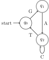
Today we talked about nondeterministic pushdown automata (NDPA) which are basically just NFAs with a stack. We started with this example:

This NDPA accepts the language $L = \{a^n b^n : n \in \mathbb{N}\}$. Notice that each arrow has three parts, for example the first loop is labeled $a, \epsilon/a$ which means you can take this loop if you read an $a$ from the input string, and pop $\epsilon$ (i.e., nothing) from the stack, and then push $a$ onto the stack. We will always use this notation (read, pop/push) for each arc.

NDPAs work just like NFAs, except they have this extra rule: You only accept a string if you finish in an accepting state and the stack is empty.

Some things to note:

1. Since the machine is nondeterministic, you can have more than one state (and more than one stack) branching off whenever you have a choice about which arrow to take.

2. If you are in a state and there is no valid arrow to take, then that state dies.

We looked at these questions:

1. For the NPDA below, describe the language that it accepts.
   

   

2. Describe an NPDA that accepts the language $L = \{ a^n b^m : n \ge m \}$.

3. Describe an NPDA with just one state that accepts the language of balanced parentheses.

Wednesday, October 4

Today we talked about the equivalence between CFGs and NPDAs. We sketched the proof of one direction: that if you have a CFG, then there is an NPDA that accepted the same language.

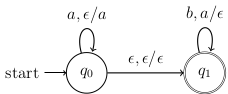
The idea of the proof is to create an NPDA with three states. In state $q_0$ you immediately transition to $q_1$ reading nothing and push S$ on the stack (where $ is a special symbol to mark the bottom of the stack). Then in state $q_1$ you have two different types of transitions that loop back to $q_1$:

1. Transitions where you read nothing and pop a variable off the stack, then push the output of one of the grammar rules for that variable back onto the stack. (I called these red transitions.) You have one red transition for each of the rules in the grammar.

2. Transitions where you read a symbol from the input and pop that symbol off the stack. (I called these blue transitions.) You have one blue transition for each of the terminals in the grammar.

Finally, you have a final transition to the accepting state $q_2$ which involves reading nothing and popping the $ off the stack. If you have finished reading the input when you do this, you will accept the string.

We illustrated how this idea works using the grammar and the input string aabbbb.

    S →  AB
    A →  aAb | ε
    B →  bB | b

We finished by describing how Deterministic Pushdown Automata (DPDAs) are different from Nondeterministic Pushdown Automata (NPDAs) and the hierarchy of different languages that we have seen so far. We looked at this example DPDA:

Friday, October 5

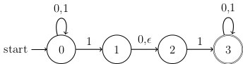
Today we introduced Turing machines (TMs) which will be the most general model of computation that we will discuss. We looked at two examples of TMs:

1. First we drew a state diagram for a TM that accepts the language $\{w=w : w \in \{a,b\}^* \}$.

2. Second we described an algorithm for a TM that accepts the language $\{a^{2^n} : n \ge 0\}.$

We defined what it means for a Turing machine to accept or recognize a language if it accepts every string in the language. We also defined when a Turing machine decides a language, and how that is different than just accepting/recognizing. Both of the example Turing Machines above actually decide their languages, since they will successfully reject any input that doesn’t match a valid string (they won’t get stuck running forever without halting).

Week 8 Notes

Monday, October 9

Today we started with this example:

1. Construct a Turing machine that reads an input string $w \in \{a,b\}^*$ and leaves $ww$ on the tape when it halts.

This wasn’t to hard to describe the algorithm, but it got a little complicated when we made the state diagram. Once we did that, we defined Turing computable functions.

Definition. A function $f: \Sigma^* \rightarrow \Sigma^*$ is Turing computable if there is a Turing machine that halts with $f(w)$ on the tape whenever it is given a tape with $w \in \Sigma^*$ as input.

2. Explain why the function $f(w) = wwww$ is Turing computable.

3. Prove that if $f, g : \Sigma^* \rightarrow \Sigma^*$ are both Turing computable functions, then so is the composition $f \circ g$.

4. Explain why the function $$f(w) = \begin{cases} 1 & \text{ if length of } w \text{ is even.} \\ 0 & \text{ otherwise.} \end{cases}$$ is Turing computable. Hint: Every regular language is Turing decidable.

We finished by describing how this function (which comes up in the Collatz-Conjecture) is Turing computable: $$f(n) = \begin{cases} n/2 & \text{ if } n \text{ is even,} \\ 3n+1 & \text{ if } n \text{ is odd.} \end{cases}$$

Wednesday, October 11

Today we mentioned but did not prove that any problem that a multi-tape Turing machine can solve, can also be solved by a single-tape Turing machine. You can find a readable proof in Section 4.3 in the book.

Instead, we summarized what we know so far:

1. Turing machines are able to decide any regular or context-free language. That is, if $L \subset \Sigma^*$ is a context-free language, then the function $f: \Sigma^* \rightarrow \{0,1\}$ defined by $f(w) = 1$ if and only if $w \in L$ is Turing computable.

2. If $f$ and $g$ are Turing computable functions, then so is the composition $f \circ g$.

3. If $f: \Sigma^* \rightarrow \{0,1\}$, and $g, h: \Sigma^* \rightarrow \Sigma^*$ are Turing computable, then so is the function

   IF f(x) THEN g(x) ELSE h(x).

4. So here is a question: Can a Turing machine have a for-loop, where it repeats some function $n$ times? Something like this Python example where function $f$ is applied $n$ times?

for i in range(n): 
    x = f(x)

2. What about a while-loop?

while(f(x)):
    x = g(x)

I think we get the idea that you can implement pretty much all of the basic building blocks of most programming languages using Turing machines. There are many other models of computing that can be proven to be Turing complete, that is, they can compute the same functions as Turing machines. But it is believed that there is no “effective method” of computation that can solve problems that Turing machines cannot solve. The Church-Turing thesis says that an computational task that we can describe how to solve with an algorithm can be computed by a Turing machine.

We finished by discussing Hilbert’s 10th problem: Is there an algorithm to determine whether a multivariable polynomial with integer coefficients has an integer root. We looked at some example polynomials like $$p(x,y) = (x-1)^2 + (y-3)^2 = x^2 + y^2 - 2x - 6y + 10$$ and $$q(x,y) = x^2 + y^2 - 2x - 6y + 11.$$ It turns out that no Turing machine can decide the language of integer multivariable polynomials with integer roots. But we did describe an algorithm that recognizes that language.

Friday, October 13

Today we introduced enumerators. An enumerator for a language $L \subseteq \Sigma^*$ is a Turing machines that computes a function $f: \mathbb{N}\rightarrow L$ that is onto. We started by proving the following:

“Easy” Lemma. If $L \subset \Sigma^*$ is decidable, then there is an enumerator for $L$.

To prove this lemma, we came up with the following algorithm. In class I didn’t include the just_started variable which caused a minor issue in the proof.

input n
# use a decider function to return the n-th string in the language
s = ""
for i in range(n):
    just_started = True
    while just_started or not decider(s):
        just_started = False
        increment(s)
return s

“Harder” Theorem. A language $L \subset \Sigma^*$ is recognizable if and only if there is an enumerator for $L$.

It was relatively easy to prove the $(\Leftarrow)$ direction as this algorithm demonstrates:

input w
# use an enumerator function to return True if w is in L
n = 0
while not w == enumerater(n):
    n++
return True

The other direction is harder to prove. We sketched a proof at the board, but the important thing to understand is this: Why doesn’t the algorithm for the “Easy Lemma” prove the $(\Rightarrow)$ case of the “Harder Theorem”?

Week 9 Notes

Wednesday, October 18

Today we introduced universal Turing machines. We use them to consider this language:

$$\text{Accept} = \{ \langle M, w \rangle : M \text{ is a Turing machine and } w \text{ is a string that } M \text{ accepts}\}.$$

1. Explain why Accept is Turing recognizable.

Then we gave a diagonalization proof that Accept is not Turing decidable. Suppose there was a decider for Accept. Then we could make a table with rows for each Turing machine $M_i$ and columns every Turing machine encoding $\langle M_j\rangle$ and entries 1 or 0 depending on whether $M_i$ accepts $\langle M_j \rangle$.

2. What would happen if we created a TM $N$ inputs any TM encoding $\langle M \rangle$ and then does the opposite of what $D$ does on $\langle M, \langle M \rangle \rangle$. What would $N$ do when you input $\langle N \rangle$ into $N$?

3. Why is that a contradiction?

We finished by observed that there are only a countably infinite number of possible Turing machines, but there is an uncountable infinite number of languages, so there must be lots of languages that are not decidable!

Friday, October 20

Today we proved that the language

$$\text{Halt} = \{ \langle M, w \rangle : M \text{ is a TM that halts on }w \}$$

is undecidable. Here is the proof:

If Halt were decidable, then we could use the following algorithm to decide if $\langle M, w \rangle \in \text{Accept}$:

1. Check if $\langle M, w \rangle \in \text{Halt}$.
2. If it is, run $M$ on $w$ and accept or reject accordingly.
3. If not, then reject.

Since this algorithm would decide the language Accept from last time, but we proved that the language Accept is undecidable, we conclude that Halt must also be undecidable.

Then we proved Rice’s theorem (our book also has a proof in Section 5.3, my proof was shorter, but I glossed over some of the details). We used Rice’s theorem to prove that these two languages are undecidable.

1. $\text{Infinte} = \{ \langle M \rangle : M \text{ is a TM and } L(M) \text{ is infinite}\}$.

2. $\text{Empty} = \{ \langle M \rangle : M \text{ is a TM and } L(M) = \varnothing \}$.

Week 10 Notes

Monday, October 23

Today we reviewed that material from CFGs and NPDAs through TMs. We did some examples:

1. Show that there is no CFG or NPDA that can generate/accept this language: $\{w w : w \in \{a,b,c\}^*\}$.

2. Find a NPDA that accepts the language $\{(ab)^n c^n : n \in \mathbb{N}\}$.

3. Use Rice’s theorem to prove that the language $\{\langle M \rangle : M \text{ is a TM that accepts } 111\}$ is undecidable.

4. Why can’t you use Rice’s theorem to prove that the language $\{\langle M \rangle : M \text{ is a TM with 3 states}\}$ is undecidable?

5. Explain why the complement of the language $$\text{HALT} = \{\langle M, w \rangle : M \text{ is a TM that accepts } w \}$$ is uncomputable (i.e., not even recognizable).

Week 11 Notes

Monday, October 30

Today we introduced big-O notation and used it to talk about running times of algorithms. Note that There are lots of important examples in Barak Chapter 12 of algorithms and their running times.

1. Which is true? $(\log n)^3 \in O(n)$ or $n \in (\log n)^3$?

We proved the following facts about big-O notation:

Theorem (Only Dominant Terms Matter). If $f: \mathbb{N}\rightarrow [0,\infty)$ is a sum of nonnegative functions $f_1, \ldots, f_k$, then there is at least one function $f_j$ such that $O(f) = O(f_j)$. We call that function a dominant term for $f$.

Theorem (Constant Multiples Don’t Matter). For any $f: \mathbb{N}\rightarrow [0,\infty)$ and constant $c > 0$, $O(cf) = O(f)$.

Theorem (Products of Functions). If $f_1 \in O(g_1)$ and $f_2 \in O(g_2)$, then $f_1f_2 \in O(g_1 g_2)$.

We also reviewed this heirarchy of functions:

$$\text{logarithms} \ll \text{polynomials} \ll \text{exponentials} \ll \text{factorials}$$

We used these ideas to find the dominant term for these expressions:

1. $n^4 + n^3 \log n + (\log n)^5$.

2. $n^{100} + 2^n$.

So why do we use big-O notation? It makes it easier to talk about a lot of formulas. For example, an algorithm that requires $7(n+3) \dfrac{n!}{k!(n-k)!}+167$ steps can be described simply as being $O(n^{k+1})$.

Caution 1. Big-O notation only gives an upper bound for how fast functions grow. Functions in $O(f)$ don’t have to grow at the same rate as $f$, they can also grow much slower.

Caution 2. You should always write the simplest possible expression inside big-O notation. For example $O(5n^3 + \log n) = O(n^3)$, so just write $O(n^3)$.

We finished by talking about how we use Big-O notation to describe the runtime of algorithms such as:

1. The TM from Midterm 2 that decrements a binary string by 1.

2. Testing whether a number $N \in \mathbb{N}$ (represented in binary) is prime.

Wednesday, November 1

Today we talked about the running times of some algorithms. We started with this example:

1. Prove that the language $\{w \in \{0,1\}^* : w \text{ is divisible by seven} \}$ can be decided in $O(n)$ time.

We defined class P which is the set of all decidable languages $L$ for which there exists a Turing machine $M$ and a constant $k \in \mathbb{N}$ such that $M$ can decide $L$ in $O(n^k)$ time.

2. Prove that if $K, L \subset \{0,1\}^*$ are both in P, then the concatenation $KL$ is also in P.

3. Consider the PATH problem which involves deciding this language: $$\text{PATH} = \{ \langle G, s, t \rangle : G \text{ is a graph containing a path from }s \text{ to } t \}.$$ Prove that the following algorithm runs in polynomial time.

   • Step 1 - place a mark on node s.
   • Step 2 - loop through the edges in the graph. For any edge that touches exactly one marked vertex, mark the other vertex.
     
   • Step 3 - repeat step 2 until you can’t find any new vertices to mark.
   • Step 4 - accept if t is marked, otherwise reject.

One important fact that I forgot to mention in class is the following:

Fact. If a Turing machine can decide a language in polynomial time, then so can a Python or C++ program.

Friday, November 3

Today we proved that all Context Free Languages (CFLs) are in class P. Before we proved this, we introduced the idea of Chomsky’s normal form. We looked at this example CFG

$$S \rightarrow aaS \,|\, \epsilon$$

and we observed that the following grammar in Chomsky normal form is equivalent, i.e., it generates the same language.

$$\begin{align*} S &\rightarrow AA \,|\, AB | \epsilon \\ A &\rightarrow a \\ B &\rightarrow AC \\ C &\rightarrow AB \,|\, AA \end{align*}$$

We did not go into the details of how to convert a CFG to Chomsky normal form, but you can find details of how to do that in Section 3.4 in Maheshwari & Smid. Instead, we did the following workshop which let us figure out the running time of an algorithm to decide whether a string of length $n$ can be generated by a grammar in Chomsky normal form.

• Workshop: Context Free Languages are in P.

Week 12 Notes

Monday, November 6

Today we introduced class NP. A language is in class NP if there is a solution string $s$ for every $w \in L$ and an algorithm called a verifier that accepts $\langle w, s \rangle$ in polynomial time in the length of $w \in L$. We looked at the following examples:

1. COMPOSITE $= \{ w \in \{0,1\}^* : w \text{ is a binary number that is not prime}\}$.

2. TRIANGLE $= \{\langle G \rangle : G \text{ is a graph with a complete subgraph with }3\text{ vertices}\}$.

In each of these examples, you need to prove that if you are given a special string called the solution, then you can find a polynomial time algorithm that will use the solution to verify that a string $w$ is in the language.

We also proved this theorem:

Theorem. P $\subseteq$ NP.

Along the way, we mentioned some interesting new results:

• 2019 Harvey & van der Hoeven Multiplication Algorithm $O(n \log n)$.
• 2003 Agarwal, Kayal, Saxena (AKS) Primality Test - polynomial time algorithm.

It is still unknown whether P $\ne$ NP.

Wednesday, November 8

Today we talked about what the name NP stands for. It refers to problems that are solvable in polynomial time by a nondeterministic Turing machine. We defined nondeterministic Turing machines, and then we proved the following:

Friday, November 10

Today we introduced the Boolean satisfiability problem (SAT). Recall that a Boolean formula/circuit (involving AND, OR, and NOT gates) can evaluate any function $f:\{0,1\}^n \rightarrow \{0,1\}$. For example, $$\phi = (\bar{x} \wedge y) \vee (x \wedge \bar{z})$$ is a Boolean formula/circuit. The Boolean satisfiability problem involves deciding if a Boolean formula can be satisfied. That is, if there are values of the input variable that can make the output TRUE. In other words, we want to decide if a Boolean formula $\phi$ is in the language $$SAT = \{ \langle \phi \rangle : \phi \text{ is a satisfiable Boolean formula} \}.$$

1. Give an example of a Boolean formula that is not satisfiable.

2. Prove that SAT is decidable.

A Boolean formula is in conjuctive normal form (CNF) if it combines a finite number of clauses made by connecting literals (either variables or negated variables) with AND statements, and then the clauses are all joined together by OR statements. For example
$$\phi = (\bar{x} \wedge y) \vee (x \wedge \bar{z})$$ is in CNF.

An important special case of the SAT problem is the 3SAT problem, which only looks at Boolean formulas in CNF where the clauses each involve only 3 literals. So a 3-CNF formula would be something like: $$(x_1 \vee \bar{x_2} \vee x_3 ) \wedge (\bar{x_3} \vee x_5 \vee x_6 ) \wedge (\bar{x_3} \vee x_6 \vee \bar{x_4}) \wedge (x_4 \vee x_5 \vee x_6 ).$$

3. If a Boolean formula has $n$-variables, then how many different 3-clauses are possible?

Instead of using a brute force algorithm to decide 3SAT, we will take a different approach and prove that solving the 3SAT problem is not much harder than deciding this language:

$$\text{CLIQUE} = \{ \langle G, k \rangle : G \text{ is a graph with a } k\text{-clique} \}.$$

4. Prove that CLIQUE is in class NP.

The key to link 3SAT and CLIQUE is to draw a graph where every vertex corresponds to a literal in one of the clauses, and we draw edges according to the following rules:

• Never draw an edge connecting literals in the same clause.
• Always draw an edge connecting literals in different clauses, unless they are negations of each other.

Then, if a Boolean formula in 3-CNF has $k$-clauses, then it is decidable iff the corresponding graph has a $k$-clique (as the following image illustrates):

Week 13 Notes

Monday, November 13

Today we introduced polynomial time reductions.

We started by proving that SAT $\le_P$ 3SAT. To prove that we considered the following transformation:

For any clause $(x_1 \vee \bar{x}_2 \vee x_3 \vee \bar{x}_5 \vee x_6 \vee x_8)$, you can replace the last two literals by a dummy variable $d_1$ and then add another clause with $\bar{d}_1$ and the two literals you removed.

1. Explain why this transformation will preserve whether or not a boolean formula in CNF is satisfiable.

2. Explain why this transformation can be computed in polynomial time.

We looked at this theorem:

3. Give an algorithm proof for this theorem.

We also proved that 3SAT $\le_P$ CLIQUE by looking at how long it takes to construct the graph in the example from last class. We finished by defining NP-complete.

Wednesday, November 15

Today we went over Homework 10. We didn’t cover any new material, but we did introduce the following language:

$$\text{FIB} = \{w \in [0-9]^* : w \text{ is a decimal representation of a Fibonacci number} \}.$$

So FIB contains $\{1,2,3,5,8,13,21,34,55,\ldots\}$.

Then we asked whether the following decimal strings are in FIB$^*$:

• 123
• 89134
• 994412

We also determined that FIB $\in$ P since the following algorithm runs in less than $O(n)$ time:

Fib = [1,1]
while w < Fib[-1]:
    Fib.append(Fib[-2]+Fib[-1])
if w == Fib[-1]:
    return true
else: 
    return false

Friday, November 17

Today I started by announcing this extra credit project. You can do it on your own, or bring your laptop to class on Monday and we’ll work on it then.

Then we introduced the classes NP-complete and NP-hard.

We prove that the relationship $\le_P$ (polynomial-time reducibility) is transitive, and used that to prove this theorem:

1. Prove that if $A \le_P B$ and $B \in \text{P}$, then $A \in \text{P}$.

We finished by talking about the Cook-Levin theorem

We sketched a proof. First we observe that for any $A \in \text{NP}$ there is a polynomial time verifier $V$ that can decide if $w \in A$ with the help of a solution string $s$. Assuming that both $w$ and $s$ are encoded in $\{0,1\}^*$, we can reduce the question of whether $w \in A$ to a question about whether there is a solution $s \in \{0,1\}^{n^k}$ such that $V$ accepts $\langle w, s \rangle$. If we think of $w$ as fixed, then the question of whether there is a solution is equivalent to asking whether the Boolean function

$f(s) = \begin{cases} 1 & \text{ if } V \text{ accepts } \langle w, s \rangle \\ 0 & \text{ otherwise.} \end{cases}$

is satisfiable.

Since that question is a Boolean function $f: \{0,1\}^{n^k} \rightarrow \{0,1\}$, there is a Boolean formula involving AND, OR, and NOT for $f$. We just have to prove that we can construct that formula in polynomial time.

To prove that you can construct a formula for $f$ in polynomial time, observe that $V$ only has a finite number of states which can be described by a state string $q \in \{0,1\}^m$. There is also exactly one position on the tape that the head is pointing to at a time. Call that position the head variable $h$. Since at each step $V$ reads the head variable, writes a new value for the head variable and then moves to a new state, while moving the head variable left or right on the tape, you can create a Boolean formula to simulation the action of one step of $V$ on $q$ and $h$ in constant time. Then each step will correspond to a different Boolean formula with the same state variable $q$ but possibly different head variables. After $O(n^k)$ steps, the verifier will accept or reject, so we can create a Boolean formula to simulate $V$ in $O(n^k)$ time.

Monday, November 20

Today we talked about homework 11. We also talked about the extra credit project. In particular, I suggested that the following hint might help write an algorithm to solve problem 3 from homework 10:

Week 14 Notes

Monday, November 27

Today we focused on review for the midterm on Wednesday. The midterm will cover the following topics:

• Big-O notation
  • You should be able to describe simple polynomial time algorithms and identify the Big-O run-time for an algorithm involving loops.
• Classes P vs. NP
  • understand the definitions of these two classes.
  • For NP languages, you should be able describe a verifier algorithm and explain why it runs in polynomial-time.
  • Should also understand the difference between a verifier algorithm and a nondeterministic polynomial-time decider.
    
• Polynomial time reductions
  • understand polynomial-time reductions and be able to describe simple examples.
• NP-complete & NP-hard
  • understand the definitions and be ready to prove basic facts like what was in the homework.
• SAT problem & Cook-Levin theorem
  • memorize these.

1. Factoring large integers is hard (it can be done in nondeterministic polynomial time, but most computer scientists believe it cannot be done in polynomial time). For example, the integer 82264459 factors as (9049)(9091). Explain the difference between a function that factors an integer and a function that can verify if a factorization is correct. What would the two functions input? Why would the later function definitely run in polynomial time even if the first function cannot?

2. A language is in class EXP if it can be decided in $O(2^{(n^k)})$ time for some integer $k$. Prove that $\text{NP} \subseteq \text{EXP}$. Note: It is an open problem whether or not $\text{NP} = \text{EXP}$.

3. Explain why the problem of finding the median entry in an array of integers is polynomial time reducible to the problem of sorting an array of integers.

We also reviewed some of questions from HW11. In particular, we talked about problem #4 and how you can write a polynomial time nondeterminsitic algorithm by including a random number generator in your pseudocode. Then if any of the random results accepts the input, then the whole algorithm does.

Friday, December 1

Today we reviewed the Chomsky heirarchy of languages, and we looked at how the different complexity classes (P, NP, EXP) fall in that heirarchy. We also review problem 2 from the midterm. We also did the following exercise in class:

1. Prove that $\text{HALT} = \{ \langle M, w \rangle : M \text{ halts on input } w \}$ is NP-Hard.

Monday, December 4

We reviewed some of the material we haven’t seen in a while. We looked at these questions.

1. Consider the regular expression 1(0|1)*(+|-)1(0|1)*. What language does this regular expression represent? Give a simple description of the strings in that language.

2. Create an NFA that recognizes that language.

3. Since the language is regular, it is also context free. Create a context free grammar that generates the language.

4. Consider the language $L = \{ w - w = 0 : w \text{ is any binary number}\}$. Prove that this language is not context free. (Use the pumping lemma for CFLs).

5. Show that the language $L$ from the previous problem is decidable by describing a Turing machine algorithm that can decide $L$. What is the run-time for that algorithm in big-O notation?

6. What is an example of a language that is context free but not regular?

7. Describe an NPDA that recognizes your language from the previous question.