Complex Analysis Notes

Math 444 - Spring 2023

• Class Notes
• Schedule & Syllabus
• Software

Jump to week: 1, 2, 3, 4, 5, 6, 7, 8, 9, 10, 11, 12, 13, 14

Week 1

Tentative Schedule

Monday, Jan 16

We did these exercises in class.

1. Simplify $\displaystyle\frac{1}{4+3i}$ by rationalizing the denominator.

The next two problems can be solved using either rectangular or polar form:

2. Find $(1+i)^2$.

3. Find $\dfrac{1}{1+i}$.

Finally, some problems are definitely easier using polar form:

4. Find $\sqrt{-i}$.

Wednesday, Jan 18

Today we derived the angle addition formulas in trigonometry from Euler’s formula. We also looked at some other trigonometry facts like the double and triple angle formulas and the law of cosines.

Friday, Jan 20

On Friday, we talked about sets of complex numbers and how multiplication by a complex number $z = R e^{i \theta}$ stretches a set by a factor of $R$ and rotates the set by an angle of $\theta$ (in the counter-clockwise direction). We also talked about the triangle inequality which says that $$|z \pm w| \le |z|+|w|$$ for any two complex numbers $z$ and $w$.

Week 2 Notes

Tentative Schedule

Monday, Jan 23

Today we talked about topology which is the study of how sets are connected. We defined the following: neighborhoods, interior points, open sets, closed sets, interiors, closures, and boundaries. These are all standard definitions (which are in the book).

We also defined the following which is not in the book:

A set $A \subseteq \mathbb{C}$ touches a point $z \in \mathbb{C}$ if every neighborhood of $z$ contains an element of $A$. Then a set is closed if it contains every element it touches.

We used the notion of touch to define continuous functions. We finished by talking about paths which are continuous functions from an interval $[a,b]$ to $\mathbb{C}$.

Wednesday, Jan 25

We talked a little more about topology, including bounded sets and path connected sets. Then we looked at using Python to work with complex numbers.

• https://colab.research.google.com/drive/1YzqxHL_l3-Uf0Rt0Za6yBWkef7ax8Fug?usp=sharing

Friday, Jan 27

On Friday we did this workshop about sequences and continuity. We did #1-3 in class.

• Workshop: Sequences and Convergence

Week 3 Notes

Tentative Schedule

Monday, Jan 30

We proved that the product of two continuous functions is continuous. We also talked about how to calculate limits of complex functions and we did these examples:

1. $\displaystyle\lim_{z \rightarrow i} z^2$.

2. $\displaystyle\lim_{z \rightarrow 0} \dfrac{z}{\overline{z}}$.

3. Exercise 2.6.

Wednesday, Feb 1

Today we talked about derivatives of complex functions. We did the following examples:

1. Use the definition to find the derivative of $z^2$.

2. Show that the derivative of $f(z) = \overline{z}$ does not exist.

We talked about properties of the derivative including the power rule, chain rule, product rule, and quotient rule. Then we talked about the meaning of the derivative in terms of linear approximations using these two apps:

• Complex function visualizer. This is a cool web app made by Alex Wang to show how a complex function f:ℂ→ℂ transforms shapes in the complex plane.
• Another complex function visualizer. This is a web app that I hacked together inspired by the Alex Wang’s.

Friday, Feb 3

On Friday, we talked about the Cauchy-Riemann Equations. Here is a nice video explanation:

• https://youtu.be/BvvFdmOrob4

In class we calculated the Cauchy-Riemann equations for the following examples to see whether they are (complex) differentiable:

1. $f(z) = z^2$.

2. $f(z) = \overline{z}$.

Week 4 Notes

Tentative Schedule

Monday, Feb 6

Today we talked more about the Cauchy-Riemann equations. We looked at two examples:

1. $f(z) = e^z$

2. This is Exercise 2.19 in the book: Define $f(z) = 0$ if $z$ is on either purely real or purely imaginary, and $f(z) = 1$ otherwise. Show that $f$ satisfies the Cauchy–Riemann equations at $z = 0$, yet $f$ is not differentiable at $z = 0$. Why doesn’t this contradict the theorem about a complex function being complex differentiable if and only if it satisfies the Cauchy-Riemann equations?

Then we talked about smooth paths which are paths that are differentiable. If $\gamma$ is a smooth path in $\mathbb{C}$ and $f$ is holomorphic, then the chain rule holds and says that $$\displaystyle\frac{d}{dt} f(\gamma(t)) = f'(\gamma(t)) \cdot \gamma'(t).$$

1. Find the derivative of the path $\gamma(t) = e^{it}$. What does it mean?

2. If $f(z) = z^2$ and $\gamma(t) = t^2 + i t$, then find the derivative of the path $f(\gamma(t))$ at $t=1$.

Then we proved that if $f$ is holomorphic on a connected open set $G$ and $f'(z) = 0$ everywhere on $G$, then $f$ must be constant.

Wednesday, Feb 8

Today we reviewed Homework 3. We also talked about the function $f(z) = \sqrt{z}$. This lead to a discussion of the principal branch of the square root function, and the idea of a branch cut.

Friday, Feb 10

Today we introduced Möbius transformations and talked about how they transform lines and circles into lines and circles.

Week 5 Notes

Tentative Schedule

Monday, Feb 13

Today we talked more about Möbius transformations. We proved that you can compose two Möbius transformations by multiplying their coefficient matrices. We also talked about the extended complex plane $\mathbb{C} \cup \{ \infty \}$. A Möbius transformation is a one-to-one and onto map from the extended complex plane to itself. Furthermore, a Möbius transformation is completely defined by what it does to any three elements of $\mathbb{C} \cup \{ \infty \}$.

Wednesday, Feb 15

We introduced the complex sine and cosine functions and the complex logarithm.

Friday, Feb 17

We talked about the principle branch of the complex power function $z^\alpha$.

Week 6 Notes

Tentative Schedule

Monday, Feb 20

Today we wrapped up our discussion of logarithms, exponentials, and power functions. We proved the following in class:

1. If $z \in \mathbb{C}$, then $\overline{(e^z)} = e^{\overline{z}}$.

2. If $z \in \mathbb{C}\backslash \{0 \}$, then $\overline{\operatorname{Log}(z)} = \operatorname{Log}(\overline{z})$.

As a consequence, it follows that for any complex $z, \alpha \in \mathbb{C}$, $\overline{z^\alpha} = \overline{z}^\overline{\alpha}$. Not every complex function commutes with the conjugate function. In fact, we showed that:

3. In order for a function $f: \mathbb{C}\rightarrow \mathbb{C}$ to commute with complex conjugation, it is necessary that $f(\mathbb{R}) \subseteq \mathbb{R}$.

We also looked at Problem #7 from HW6. And we finished with this exercise:

4. What is the image of the square with corners $0, i, 1,$ and $1+i$ under the function $f(z) = e^z$?

Week 7 Notes

Tentative Schedule

Monday, Feb 27

Today we introduced complex integrals. We did these examples:

1. $\displaystyle\int_\gamma (\overline{z})^2 \, dz$ on the path $\gamma(t) = t(1+i)$ with $t \in [0,1]$.

2. $\displaystyle\int_\delta (\overline{z})^2 \, dz$ on the path $\delta(t) = t+it^2$ with $t \in [0,1]$. (Link: Sympy code)

3. $\displaystyle\int_\gamma \frac{1}{z} \, dz$ where $\gamma$ is the unit circle $\gamma(t) = e^{it}$ with $t \in [0,2\pi]$.

4. Use the formula $\displaystyle\operatorname{length}(\gamma) = \int_a^b |\gamma'(t)| \, dt$ to find the length of the unit circle.

5. Use the formula $\displaystyle\left| \int_\gamma f(z) \, dz \right| \le \max_{z \in \gamma} |f(z)| \cdot \operatorname{length}(\gamma)$ to estimate an upper bound for $\displaystyle\left| \int_\gamma \frac{1}{z^4 + 16} \, dz \right|$ when $\gamma$ is the unit circle.

Friday, Mar 3

Today we proved Cauchy’s Theorem using Green’s Theorem (see this video for a nice explanation of Green’s theorem).

Cauchy’s Theorem: If $f$ is holomorphic on a simply connected open set $D \subseteq \mathbb{C}$, and $C$ is a (piecewise smooth) simple closed path in $D$, then $$\oint_C f(z) \, dz = 0.$$

As a corollary, we showed that when a function $f(z)$ is holomorphic on a simply connected open set $D$, then the integral on any two paths $\gamma_1$ and $\gamma_2$ that both start at a point $z_0$ and end at $z_1$ and stay inside $D$ must be the same:

$$\int_{\gamma_1} f(z) \, dz = \int_{\gamma_2} f(z) \, dz.$$

In other words, the value of the integral is independent of the path.

Week 8 Notes

Tentative Schedule

Monday, Mar 13

Today we reviewed Cauchy’s theorem. We pointed out that many of the assumptions we made last time aren’t really necessary. The general version of Cauchy’s theorem says:

Cauchy’s Theorem. Let $f$ be holomorphic on a simply connected open set $D \subseteq \mathbb{C}$. Then $$\oint_C f(z) \, dz = 0$$ for every piecewise smooth closed path $C$ in $D$.

Our proof using Green’s theorem required extra assumptions that aren’t really necessary, but without them the proof gets more complicated:

1. We assumed that $f'$ is continuous.
2. We assumed that our paths were simple.

We reviewed consequences of Cauchy’s theorem like path independence of integrals. Then we defined an antiderivative of a complex function. If you know $F$ is an antiderivative of $f$ and $\gamma: [a,b] \rightarrow \mathbb{C}$ is a piecewise smooth path, then the evaluation theorem says that $$\int_\gamma f(z) \, dz = F(\gamma(b)) - F(\gamma(a)).$$

We finished by proving that any holomorphic function $f$ on a simply connected open set $D$ always has an antiderivative. If the domain $D$ is not simply connected, then you have to assume that $f$ is continuous and the integral of $f$ on any closed path in the domain is 0 (see Theorem 4.15 in the book).

Wednesday, Mar 15

Today we introduced the Cauchy integral formula which extends Cauchy’s theorem. The proof required two key insights:

1. If $f$ is complex differentiable at $w$, then $$f(z) = f(w) + f'(w) (z-w) + \epsilon(z),$$ where the error term $\epsilon(z)$ satisfies $\lim_{z \rightarrow w} \frac{\epsilon(z)}{z-w} = 0$.

2. If $C_1$ and $C_2$ are two different positively oriented piecewise smooth closed paths in a region where $f$ is holomorphic, then $$\int_{C_1} \frac{f(z)}{z-w} \, dz = \int_{C_2} \frac{f(z)}{z-w} \, dz.$$

Then we used the Cauchy integral formula to evaluate the following integrals.

1. $\displaystyle\int_C \frac{e^z}{z-1} \, dz$ where $C$ is the square with vertices at $10, 10i, -10, -10i$. (https://youtu.be/NJap6Vm5mEk)

2. $\displaystyle\oint_{|z-i|=1} \frac{1}{z^2+1} \, dz$

3. $\displaystyle\oint_{|z|=3} \frac{e^z}{z^2 - 2z} \, dz$

Friday, Mar 17

We started by proving the geometric sum formula: $1 + z + z^2 + \ldots = \frac{1}{1-z}$ for any $z \in \mathbb{C}$ with $|z| < 1$. Then use that to prove this:

Theorem If $f$ is holomorphic in an open set containing a closed disk $B_R(z_0)$, then $f(z)$ has a power series $f(z) = \sum_{n = 0}^\infty a_n (z-z_0)^n$ which converges absolutely inside the disk $B_R(z_0)$. The coefficients of the power series are $$a_n = \frac{1}{2\pi i} \oint_{|\xi-z_0|=R} \frac{f(\xi)}{(\xi-z_0)^{n+1}} \, d\xi.$$

In the special case where $z_0 = 0$ you get a Maclaurin series with coefficients: $$a_n = \frac{1}{2\pi i} \oint_{|\xi|=R} \frac{f(\xi)}{\xi^{n+1}} \, d\xi.$$ This follows from Cauchy’s integral formula and the geometric series formula $$f(z) = \frac{1}{2\pi i} \oint_{|\xi|=R} \frac{f(\xi)}{\xi - z} \, d\xi = \frac{1}{2\pi i} \oint_{|\xi|=R} \frac{f(\xi)}{\xi} \left( \sum_{n = 0}^\infty \frac{z^n}{\xi^n} \right) \, d\xi.$$

Note that the coefficients are all bounded in absolute value by $\displaystyle\max_{|\xi|=R} \frac{|f(\xi)|}{R^n}$ so the series does converge absolutely as long as $|z| < R$.

Week 9 Notes

Tentative Schedule

Monday, Mar 20

Today we talked about Cauchy’s integral formula for derivatives. We did these examples in class:

1. $\displaystyle\oint_{|z| = 3} \frac{e^{iz}}{(z+i)^2} \, dz$. (https://youtu.be/WJOf4PfoHow)

2. $\displaystyle\oint_{|z| = 1} \frac{z^2+1}{z(2z+1)} \, dz$. (https://youtu.be/APoh2B5S2ok)

We finished by using a complex contour integral to find the real integral $\displaystyle\int_{-\infty}^{\infty} \frac{1}{x^4+1} \, dx$.

Wednesday, Mar 22

Today we talked about two theorems:

Morera’s Theorem If $f:D \rightarrow \mathbb{C}$ is continuous in an open connect set $D \subseteq \mathbb{C}$, and $\int_\gamma f(z) \, dz = 0$ for every piecewise smooth closed path $\gamma$ in $D$, then $f$ is holomorphic.

In class last week we proved that the functions described above have a well-defined antiderivative function $F$. But then, Cauchy’s general integral formula guarantees that $F$ is holomorphic, and so are all of its derivatives, including $f$!

Then we looked at another interesting concept:

Definition The winding number of a closed curve $\gamma$ around a point $z_0 \in \mathbb{C}$ $$\frac{1}{2\pi i} \int_\gamma \frac{1}{z-z_0} \, dz$$ (assuming that $\gamma$ does not intersect $z_0$).

Theorem If $p(z)$ is a polynomial with no roots on the unit circle, then the winding number of $p(e^{it})$ around the origin is equal to the number of roots of $p$ inside the unit circle.

We proved this theorem by doing the following exercises in class:

1. If $\gamma(t) = p(e^{it})$, show that $\displaystyle\int_\gamma \frac{1}{z} \, z = \oint_{|z|=1} \frac{p'(z)}{p(z)} \, dz$.

2. If $f(z) = (z-w)^m g(z)$ where $g(z)$ is holomorphic and $g(w) \ne 0$ in a disk of radius $R$ around $w$, then $\displaystyle\frac{1}{2\pi i } \oint_{|z-w| = r} \frac{f'(z)}{f(z)} \, dz = m$ for any $0 < r< R$.

Friday, Mar 24

Today we finished the proof of the theorem from Wednesday. We observed that for a polynomial $p(z) = (z-r_1)^{m_1} (z-r_2)^{m_2} \cdots (z-r_k)^{m_k}$, the winding number of $\gamma(t) = p(e^{it})$, $0 \le t \le 2 \pi$ around the origin will be $$\frac{1}{2\pi i} \oint_\gamma \frac{1}{z} \, dz = \frac{1}{2\pi i} \oint_{|z|=1} \frac{p'(z)}{p(z)} \, dz = \sum_{|r_j|<1} m_j.$$

Then we talked about entire functions which are functions that are holomorphic everywhere in $\mathbb{C}$.

Liouville’s Theorem. Any bounded entire function is constant.

To prove Liouville’s theorem, we need a quick observation and an idea. The observation is that if $f'(z) = 0$ everywhere, then $f$ must be constant. The idea is that we can use Cauchy’s integral formula for derivatives to calculate $f'(z)$ if $f$ is bounded and entire: $$f'(z) = \frac{1}{2\pi i} \oint_{|\xi - z| = R} \frac{f(\xi)}{(\xi - z)^2} \, d\xi.$$ What happens if the radius $R$ gets really really big? Use the max-times-length inequality to estimate $|f'(z)|$.

We finished by applying Liouville’s theorem to prove:

The Fundamental Theorem of Algebra Every nonconstant polynomial with complex coefficients has a complex root.

Week 10 Notes

Tentative Schedule

Monday, Mar 27

Today we gave a completely different proof of the Fundamental Theorem of Algebra by thinking comparing the contour $p(Re^{i t})$ when the radius $R$ is small versus when it is large. Here is a video that explains the proof we did:

• Numberphile video about Fundamental Theorem of Algebra.

Before we did that, we reviewed some facts about polynomials.

Rational Root Theorem. If $p(z) = a_n z^n + \ldots + a_1 z + a_0$ has integer coefficients, then any rational root of $p$ must be expressed as a reduced fraction $\frac{m}{d}$ where $m$ divides $a_0$ and $d$ divides $a_n$.

We used the rational root theorem to check the possible rational roots of $p(z) = z^3 - 3z^2 + z - 3$. We found that $z = 3$ is a root.

Division Algorithm for Polynomials. If $p(z)$ and $d(z)$ are polynomials with complex coefficients and $\operatorname{degree}(d) > 0$, then there are unique polynomials $q(z)$ and $r(z)$ with $\operatorname{degree}(r) < \operatorname{degree}(d)$ such that $$p(z) = q(z) d(z) + r(z).$$

In particular, this means that $z^3 - 3z^2 + z - 3 = (z-3)(z^2 + 1) + \text{ a remainder}$. But since $3$ is a root, it is clear that the remainder must be zero. So $(z-3)$ is on factor. Factoring $(z^2+1)$, we see that $$z^3 - 3z^2 + z - 3 = (z-3)(z - i)(z+i).$$ In general, we have the following corollary of the Fundamental Theorem of Algebra:

Theorem. An n-th degree polynomial $p(z) = a_n z^n + \ldots + a_0$ with complex coefficients always factors into the form $$a_n(z-r_1) (z-r_2) \cdots (z-r_n)$$ where reach $r_k$ is a root of $p(z)$ (repeats are allowed).

We used these ideas to completely factor these two polynomials:

1. $p(z) = z^3 - 3z^2 + z - 3$

2. $p(z) = z^3 + 1$

Wednesday, Mar 29

We started by proving this theorem which effectively says that $f(w)$ is the average of the values of $f$ in a circle around $w$:

Theorem. If $f$ is holomorphic in a region that contains a closed disk $\overline{B_R}(w)$, then $$f(w) = \frac{1}{2\pi} \int_0^{2\pi} f(w + R e^{i t}) \, dt.$$

After we proved that, we introduced harmonic functions which are functions $u:\mathbb{R}^2 \rightarrow \mathbb{R}$ such that $$\frac{\partial^2 u}{\partial x^2} + \frac{\partial^2 u}{\partial y^2} = 0.$$

1. Show that $u(x,y) = x^3 - 3xy^2$ is harmonic.

2. Construct a real-valued function $v(x,y)$ such that $u+iv$ satisfies the Cauchy-Riemann equations.

In fact, for every harmonic function $u$, it is always possible to construct another harmonic function $v$ such that $u+iv$ is holomorphic (at least locally). The function $v$ is called a harmonic conjugate of $u$. The converse is true as well, if $f$ is holomorphic, then both the real and imaginary parts of $f$ are harmonic functions.

Week 11 Notes

Tentative Schedule

Wednesday, Apr 5

Today we did a review of infinite series and power series. We started with the following two definitions: an infinite series converges if its partial sums converge. A series $\sum_{n = 0}^\infty a_n$ converges absolutely if $\sum_{n=0}^\infty |a_n|$ converges. We proved the following theorem:

Theorem If a series $\sum_{n = 0}^\infty a_n$ converges absolutely, then it also converges.

Then we talked about power series which are series of the form $$\sum_{n=0}^\infty a_n (z-c)^n$$ where the coefficients $a_n$ and the center $c$ are complex numbers and $z$ is a variable.

Theorem A power series $\sum_{n=0}^\infty a_n (z-c)^n$ has a radius of convergence $$R = \lim_{n \rightarrow \infty} \frac{|a_n|}{|a_{n+1}|}.$$ The power series converges absolutely for all $z$ inside the open disk with radius $R$ around center $c$. It diverges outside the closed disk of radius $R$ around $c$. On the boundary, the series might converge or diverge.

We looked at the following examples:

1. Consider the following power series for $$\operatorname{Log}(z) = (z-1) - \frac{(z-1)^2}{2} + \frac{(z-1)^3}{3} - \frac{(z-1)^4}{4} + \ldots.$$

   1. Re-write this series in $\Sigma$-notation.
   2. What are the coefficients $a_n$ of this power series?
   3. What is the center and radius of convergence?

2. Find the radius of convergence for this power series $\displaystyle\sum_{n = 0}^{\infty} \frac{z^n}{n!}$.

3. Find power series for the following functions by using the Maclaurin series for $e^z$, $\sin z$, and $\cos z$:

   1. $e^{-z^2/2}$
   2. $\dfrac{\sin z}{z}$

Friday, Apr 7

Today we reviewed some of the questions from HW10 and HW11. Then we worked on proving:

Theorem A power series $\displaystyle\sum_{n=0}^\infty a_n (z-c)^n$ converges absolutely when $$|z-c| < R = \lim_{n \rightarrow \infty} \frac{|a_n|}{|a_{n+1}|}.$$ (assuming the limit exists).

Proof. By the definition of limits, for any $\epsilon > 0$, there exists an $N$ big enough so that $$R-\epsilon < \frac{|a_n|}{|a_{n+1}|} < R+ \epsilon$$ for all $n \ge N$. This means that $$|a_{n+1}| < \frac{|a_n|}{(R-\epsilon)}$$ for all $n > N$.

Exercise. Use mathematical induction to prove that $$|a_n| \le \frac{|a_N|}{(R-\epsilon)^(n-N)}$$ for all $n \ge N$.

Now, we can choose $\epsilon > 0$ small enough so that $|z-c| < (R - \epsilon)$. Then we have $$\sum_{n = 0}^{\infty} |a_n|\, |z-c|^n = \sum_{n = 0}^{N-1} |a_n|\, |z-c|^n + \sum_{n=N}^\infty |a_n| \, |z-c|^n.$$ The first $N$ terms are not important, since they definitely have a finite sum. So we focus on the right side terms. Using the inequality from the induction exercise, we have:

$$\sum_{n = N}^{\infty} |a_n|\, |z-c|^n \le \sum_{n = N}^{\infty} \frac{|a_N|}{(R-\epsilon)^{(n-N)}} |z-c|^n.$$

That is a geometric series with common ratio $\displaystyle\left( \frac{|z-c|}{(R-\epsilon)} \right) < 1$. So it converges. □

In class I mixed up the end of the proof because I chose $\epsilon$ so that $|z-c| = R - \epsilon$ instead of $|z-c| < R - \epsilon$. That prevented the series from converging, but you can choose any $\epsilon > 0$ as small as you want, so you can definitely find one so that $|z-c| < R- \epsilon$.

Week 12 Notes

Tentative Schedule

Monday, Apr 10

Since I messed up the proof that power series converge absolutely inside their radius of convergence last Friday, I figured I’d start today be fixing the argument. But I also wanted to talk about the intuition behind the argument. To create a proof, you typically need to find an intuition for why the claim is true. Here is the intuition:

$$\sum_{n = 0}^\infty |a_n| \, |z-c|^n = |a_0| + |a_1| |z-c| + |a_2| |z-c|^2 + |a_3| |z-c|^3 + \ldots$$

Unlike geometric series, power series don’t have a common ratio. The ratio between consecutive terms here is: $$\frac{|a_{n+1}|}{|a_n|} |z-c|.$$ In the long run, this approaches $$\frac{|z-c|}{R},$$ which explains why the series will converge when $|z-c| < R$. In the long run, it behaves like a geometric series with that as its common ratio.

After that, we talked about the zeros of an analytic function. An analytic function is one with a converging power series in a disk with positive radius. Analytic functions are the same as holomorphic functions.

We proved the following theorem:

Theorem If $f$ is a non-constant analytic function in an open connected domain $D \subseteq \mathbb{C}$, then the zeros of $f$ are isolated.

This lead to the following definition. The order of a zero $z_0$ of $f(z)$ is the smallest $N$ such that the coefficient $a_N$ in the power series for $f$ centered at $z_0$ is nonzero.

Find the orders for the following zeros:

1. $z_0 = 0$ for $f(z) = z-\sin z$.

2. $z_0 = \pi i$ for $g(z) = e^z + 1$.

Week 13 Notes

Tentative Schedule

Monday, Apr 17

Today we reviewed the concept of zeros and winding numbers. We updated an old proof to show that if $\gamma:[0,2\pi) \rightarrow \mathbb{C}$ is a piecewise smooth simple closed curve in a simply connected open set where $f$ is holomorphic, then the winding number of $f(\gamma(t))$ around $w \in \mathbb{C}$ is equal to the sum of the orders of the zeros of $f-w$ that are enclosed by $\gamma$.

This is because the winding number must be equal to $$\frac{1}{2\pi i} \int_{f(\gamma)} \frac{1}{z-w} \, dz$$ by Cauchy’s integral formula. Then by the definition of complex contour integrals, this is the same as: $$\frac{1}{2\pi i} \int_\gamma \frac{f'(z)}{f(z)-w} \, dz.$$

1. Show that if $f-w$ has a zero $z_0$ of order $m$ at $w$, that is, $f(z)-w = (z-z_0)^m g(z)$ where $g$ is holomorphic and $g(z_0) \ne 0$, then $$\frac{f'(z)}{f(z)-w} = \frac{g'(z)}{g(z)} + \frac{m}{(z-z_0)}.$$

2. If $z_0$ is the only zero of $f-w$ inside $\gamma$, explain why this proves that the winding number of $f(\gamma)$ around $w$ is $m$.

3. What if $z_0$ is not the only zero of $f-w$ inside $\gamma$?

Once we finished the proof, we observed the following: If $f$ is holomorphic in a open region $R$ and $f(z)-w_0$ has a zero of order $m$ at $z_0 \in R$, then $f(\gamma)$ winds around $w_0$ exactly $m$ times when $\gamma$ is a small circle around $z_0$. Therefore $f(\gamma)$ also winds around any $w$ close to $w_0$ exactly $m$ times as well. As a corollary, we have:

Open Mapping Theorem. If $f$ is holomorphic on an open set $U \subseteq \mathbb{C}$, then $f(U)$ is an open set.

Another immediate corollary is the following theorem:

Maximum Modulus Principle. If $f$ is holomorphic on an open set $U$, then $|f|$ cannot have a local maximum in $U$.

Proof. Suppose that $z_0$ is a local maximum, that is, $|f(z_0)| \ge |f(z)|$ for all $z$ in a small disk around $z_0$. This is a contradiction because $f(B_r(z_0))$ is an open set, so it contains an open disk around $f(z_0)$. $\square$

Wednesday, Apr 19

Today we did two applications of contour integrals to calculate real integrals:

1. $\displaystyle\int_{-\infty}^{\infty} \frac{1}{(x^2-1)(x^2-9)} \, dx$.

2. $\displaystyle\int_0^{2 \pi} \frac{1}{10 - 6 \cos \theta} \, d\theta$.

To convert integrals of functions involving sine & cosine from 0 to 2π, you can use the following substitutions, all based on letting $z = e^{i \theta}$ and integrating over the unit circle:

• $d\theta = \dfrac{dz}{iz}$
• $\cos \theta = \dfrac{z + z^{-1}}{2}$
• $\sin \theta = \dfrac{z - z^{-1}}{2i}$.

Friday, Apr 21

Today we talked about the Fourier transform of a real function $f:\mathbb{R}\rightarrow \mathbb{R}$ which is defined to be:

$$\mathcal{F}(f) = \int_{-\infty}^\infty f(x) e^{i\alpha x} \, dx = F(\alpha).$$

The inverse Fourier transform is

$$\mathcal{F}^{-1}(F) = \int_{-\infty}^\infty F(\alpha) e^{-i\alpha x} \, d\alpha = f(x).$$

In class we used a contour integral to find the inverse Fourier transform of

1. $\displaystyle F(\alpha) = \frac{2}{1+\alpha^2}$

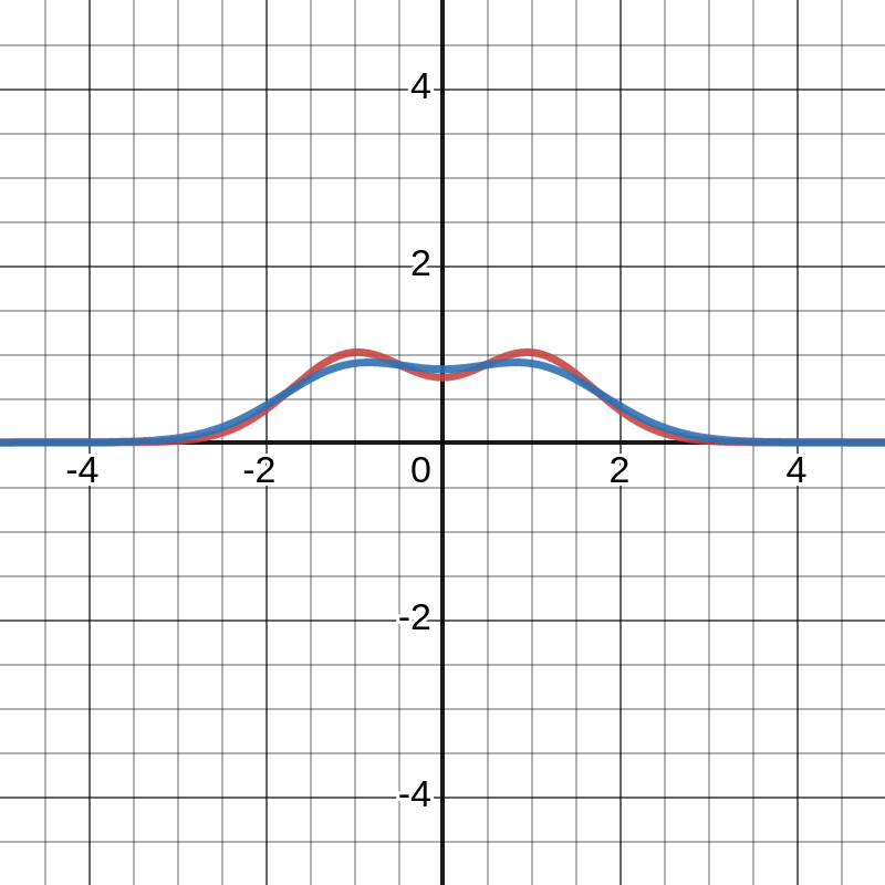
We also calculated the Fourier transform of the Gaussian $f(x) = e^{-x^2}$. Before calculating that, we needed to know that $\displaystyle\int_{-\infty}^\infty e^{-x^2} \, dx = \sqrt{\pi}$. Here is a video that explains this.

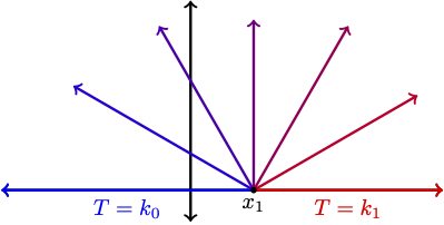
Then we used a rectangular contour to show that $\mathcal{F}(e^{-x^2}) = \sqrt{\pi} e^{-\alpha^2/4}$.

Week 14 Notes

Tentative Schedule

Monday, Apr 24

Today we used the Fourier transform to solve the 1-dimensional heat equation: $$\frac{\partial T}{\partial t} = \frac{\partial^2 T}{\partial^2 x}$$ with initial condition $T(0,x) = f(x)$.

We started with some properties of the Fourier transform. Suppose $f(x)$ is a real function with Fourier transform $\hat{f}(\alpha)$. Then we have:

1. Derivatives. $\displaystyle\mathcal{F}(f'(x)) = - i\alpha \hat{f}(\alpha)$.

2. Convolution. $\displaystyle\mathcal{F}(f \ast g) = \hat{f}(\alpha) \hat{g}(\alpha)$.

3. Scaling. $\displaystyle\mathcal{F}(f(cx)) = \tfrac{1}{|c|} \hat{f} \left( \tfrac{\alpha}{c} \right)$ and $\displaystyle\mathcal{F}^{-1}(\hat{f}(c\alpha)) = \tfrac{1}{|c|} f \left( \tfrac{x}{c} \right)$

Then we used these steps to solve the heat equation.

• Step 1. Apply Fourier transform in variable $x$ to $T$.

• Step 2. Differentiate with respect to $t$. Combined with the heat equation, you get an ordinary differential equation.

• Step 3. Solve the ordinary differential equation for $\hat{T}(t,\alpha)$.

• Step 4. Use the inverse Fourier transform to write the solution to the heat equation as a convolution of $f(x)$ and $\dfrac{1}{2\sqrt{\pi t}} e^{-x^2/4t}$.

Wednesday, Apr 26

Today we started by looking at the 2-dimensional heat equation $$\frac{\partial T}{\partial t} = \frac{\partial^2 T}{\partial x^2} + \frac{\partial^2 T}{\partial y^2}.$$

We used a contour integral with Green’s theorem to show that the next flow of heat into a disk $D$ with boundary $C$ is equal to $$\int_C \nabla T \cdot d \nu$$ where $d \nu = (dy, -dx)$ is the normal vector (times $dt$) and $\nabla T$ is the gradient of the temperature function (at a fixed time). Since the gradient points in the direction of greatest increase in temperature, the heat wants to flow in the exact opposite direction.

1. Use Green’s theorem $\displaystyle\int_C P dx + Q dy = \iint_D \frac{\partial Q}{\partial x} - \frac{\partial P}{\partial y} \, dA$ to show that the net flow of heat into $D$ is $\displaystyle\iint_D \frac{\partial^2 T}{\partial x^2} + \frac{\partial^2 T}{\partial y^2} \, dx dy$.

Steady State Solutions

When the temperature reaches equilibrium, it stops changing so the left side of the heat equation ($\partial T/ \partial t$) becomes zero. When that happens, $T = T(x,y)$ is a harmonic function. We’ve talked about functions that are harmonic on the entire complex plane. But an important problem is to find functions that are harmonic on a domain $D \subset \mathbb{C}$ that satisfy a boundary condition. This is called the Dirichlet problem.

We looked at one solution to the Dirichlet problem on the upper-half plane: $$T(z) = k_1 + \left(\frac{k_0 - k_1}{\pi} \right) \operatorname{Arg} z.$$

2. Show that the function $\displaystyle T(z) = k_1 + \left(\frac{k_0 - k_1}{\pi} \right) \operatorname{Arg} z$ is harmonic. Hint: Is there a holomorphic function with $T(z)$ as its real or imaginary part?

We finished by talking about how a harmonic function $T: D_1 \rightarrow \mathbb{R}$ that is defined on one domain $D_1 \subset \mathbb{C}$ can be turned into a harmonic function on another domain $D_2 \subset \mathbb{C}$ if you have find an invertible holomorphic function $f: D_2 \rightarrow D_1$. In that case, $T(f(z))$ is a harmonic function on $D_2$.

Friday, Apr 26

If $T$ is a harmonic function on a domain in $\mathbb{C}$, then it has a harmonic conjugate function $V$ such that $T+iV$ is holomorphic. If $T$ represents the equilibrium temperature on the domain, the what does $V$ represent?

1. Show that the level curves of $V$ are always orthogonal to the level curves of $T$. Hint: First show that the gradients of $T$ and $V$ are orthogonal.

Since the level curves of $V$ follow the direction indicated by the gradient of $T$, the level curves of $V$ represent the lines of flow for the heat at equilibrium.

We took this idea and looked at three examples of level curves and flow curves for harmonic functions:

2. We transformed the solution to the Dirichlet problem on the upper-half plane from Wednesday to a solution on the unit disk.

3. We transformed a simple linear flow along a narrow channel ($D = \{x+iy : -\pi < y < \pi\}$) to a flow escaping from the mouth of a channel using the transformation $f(z) = z+e^z$.

4. We transformed another simple linear flow (with $D = \{x+iy : -\frac{\pi}{2} < x < \frac{\pi}{2} \}$) to a flow passing through a narrow gap in the x-axis using $f(z) = \sin z$. The key to writing the transformation of the flow curves $c + it$ using $\sin z$ was to using the angle addition formulas with $\cos(it) = \cosh(t)$ and $\sin(it) = i \sinh(t)$.