Jump to week: 1, 2, 3, 4, 5, 6, 7, 8, 9, 10, 11, 12, 13, 14
| Day | Section | Topic |
|---|---|---|
| Mon, Jan 16 | 1.2 | Data tables, variables & individuals |
| Wed, Jan 18 | 2.1.3 | Histograms & skew |
| Thu, Jan 19 | 2.1.5 | Boxplots |
| Fri, Jan 20 | 2.1.5 | Boxplots - con’d |
Today we covered data tables, individuals, and variables. We collected the following data in class:
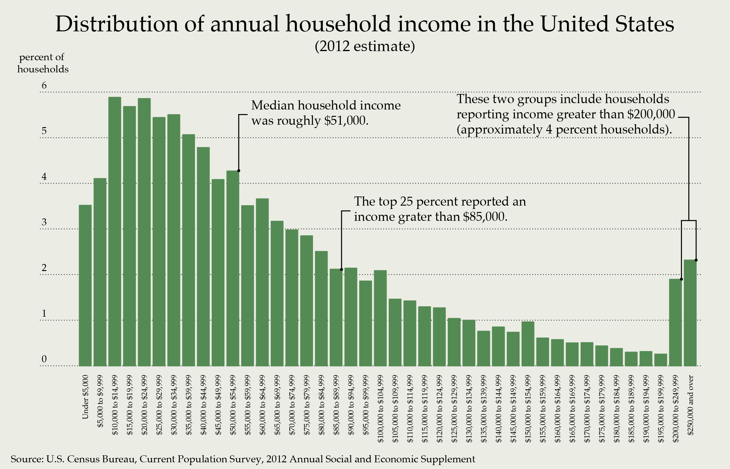
Today we talked about graphing data. We focused on stem-and-leaf plots (stemplots) and histograms. We also talked about the two measures of center: the mean and the median.
Today we talked about measures of spread in particular the interquartile range. We also talked about the five number summary and box-and-whisker plots (boxplots).
| Day | Section | Topic |
|---|---|---|
| Mon, Jan 23 | 2.1.4 | Variance and standard deviation |
| Wed, Jan 25 | 4.1 | Normal distribution |
| Thu, Jan 26 | 4.1.5 | 68-95-99.7 rule |
| Fri, Jan 27 | 4.1.4 | Normal distribution computations |
We talked about standard deviation and we introduced the normal distribution.
We talked about z-values and the 68-95-99.7 rule.
Today we talked about how to use the Probability Distributions app (android, iOS) to convert locations to percentages and vice versa on the normal distribution.
On Friday we used the app to solve the problems on this workshop:
| Day | Section | Topic |
|---|---|---|
| Mon, Jan 30 | 2.1, 8.1 | Scatterplots and correlation |
| Wed, Feb 1 | 8.2 | Least squares regression introduction |
| Thu, Feb 2 | 8.2 | Least squares regression practice |
| Fri, Feb 3 | 2.2 | Contingency tables |
On Monday we looked at scatterplots and correlation coefficients with these examples:
We also talked about explanatory and response variables.
Introduced least squares regression and started this workshop:
Today we talked about regression to the mean which is where data with extreme x-values in a scatterplot tend to have less extreme y-values.
Today we talked about two-way tables (which are called contingency tables in the book). We defined row and column proportions and we also introduced the relative risk which you calculate by dividing corresponding row or column proportions to see how many times greater the risk is in one category than in another.
| Day | Section | Topic |
|---|---|---|
| Mon, Feb 6 | 2.2 | Contingency tables Simpson’s paradox |
| Wed, Feb 8 | 1.3 | Sampling: Populations and samples |
| Thu, Feb 9 | 1.3 | Bias versus random error |
| Fri, Feb 10 | 1.4 | Randomized controlled experiments |
We talked about Simpson’s paradox which is when an apparent association between two variables reverses direction when you split up the data. We did the following example in class.
We talked about populations versus samples. A number that describes a population is called a parameter and a number that describes a sample is called a statistic. This class is all about how to use sample statistics to say something about population parameters. There are two sources of sampling error:
As an example, we each selected a sample of words chosen from the Gettysburg address. The resulting sample means showed signs of being biased. We also talked about some other examples of bias:
Then we introduced the idea of a simple random sample by using Excel to select a simple random sample from the class data.
Today we did this workshop to review the concepts from Wednesday:
We introduced randomized controlled experiments which are studies where individuals in the sample are randomly assigned to different treatment groups. This controls lurking variables which lets you establish cause and effect.
| Day | Section | Topic |
|---|---|---|
| Mon, Feb 13 | 2.3 | Simulation example |
| Wed, Feb 15 | Review | |
| Thu, Feb 16 | Midterm 1 | |
| Fri, Feb 17 | 3.1 | Defining probability |
Today we looked at an example of a randomized controlled experiment from Section 2.3 of the book. We simulated what might happen if there were no association between a vaccine and getting infected, and compared the simulation results with what actually did happen.
Today we went over the midterm 1 review problems.
Today we introduced probability models. We defined the sample space which is the set of all possible outcomes in a probability model and an event is any subset of the sample space. The probability function \(P(E)\) returns the probability that event \(E\) happens.
| Day | Section | Topic |
|---|---|---|
| Mon, Feb 20 | 3.1 | Multiplication and addition rules |
| Wed, Feb 22 | 3.2 | Conditional probability |
| Thu, Feb 23 | 3.2 | Tree diagrams and Bayes’ rule |
| Fri, Feb 24 | 3.4 | Weighted averages & expected value |
Today we talked about complementary events, the addition rule, and the multiplication rule for independent events.
Today we introduced conditional probability and weighted tree diagrams. We followed Section 3.2 in the book pretty closely, so definitely read that section!
Today we talked about weighted averages. To find a weighted average:
We also talked about random variables and expected value. A random variable is a probability model where the outcome are numbers. The expected value \(E(X)\) of a random variable \(X\) is the weighted average of the outcomes using the probabilities as the weights. The expected value is also known as the theoretical average of a random variable.
We finished by talking about the Law of Large Numbers which says: when you repeat a random experiment many times, the sample mean tends to get closer to the theoretical average.
| Day | Section | Topic |
|---|---|---|
| Mon, Feb 27 | 3.4 | Random variables |
| Wed, Mar 1 | No Class | |
| Thu, Mar 2 | 3.4 | Random variables - con’d |
| Fri, Mar 3 | 5.1 | Sampling distributions |
Today we talked about random variables which are probability models where the outcomes are numbers. We described how a random variable \(X\) has an expected value \(E(X)\) which is the theoretical mean (\(\mu_X\)) and a variance \(\operatorname{Var}(X)\) which is the theoretical standard deviation squared (\(\sigma_X^2\)).
We gave examples of continuous and discrete random variables.
We talked about how every random variable has a shape (whether it is skewed or symmetric, normal or not), a center (the theoretical mean μ) and a spread (the theoretical standard deviation σ).
Today we introduced the sampling distribution for the sample mean \(\bar{x}\). Here’s what you need to know: in a simple random sample of size \(n\) from a large population, the sample mean \(\bar{x}\) is random, so it has a probability distribution with a
Here are two examples of simulated sampling distributions:
| Day | Section | Topic |
|---|---|---|
| Mon, Mar 13 | 5.1 | Sampling distributions |
| Wed, Mar 15 | 5.1.3 | Central limit theorem |
| Thu, Mar 16 | 4.3 | Binomial distribution |
| Fri, Mar 17 | 5.2 | Confidence intervals for a proportion |
Today we talked about sampling distributions again.
We talked about sample proportions \(\hat{p}\) for categorical variables. Then we described the sampling distribution for a sample proportion which has
We did this example from the book:
Today we introduced confidence intervals for a population proportion:
\[\hat{p} \pm z^* \sqrt{ \frac{\hat{p}(1-\hat{p})}{N}}.\] The number \(z^*\) is called the critical z-value and it is determined by the confidence level you want:
| Confidence Level | 90% | 95% | 99% | 99.9% |
|---|---|---|---|---|
| Critical z-value | 1.645 | 1.96 | 2.576 | 3.291 |
Every confidence interval has two parts: the best guess estimate which is the number before the ± symbol, and the margin of error which is the number after the ± symbol. We did these examples:
Use data in Exercise 5.4 to make a 95% confidence interval for the percent of all Americans who can’t afford a surprise $400 expense.
Use the class data to make a 95% confidence interval for the percent of all HSC students who were born in VA.
In 2004 the General Social Survey found 304 out 977 Americans always felt rushed. Find the margin of error for a 90% confidence interval with this data.
| Day | Section | Topic |
|---|---|---|
| Mon, Mar 20 | 5.2 | Confidence intervals for a proportion - con’d |
| Wed, Mar 22 | Review | |
| Thu, Mar 23 | Midterm 2 | |
| Fri, Mar 24 | 5.3 | Hypothesis testing for a proportion |
Today we went over the review problems for midterm 2.
Today we introduced hypothesis testing. We talked about the difference between the null hypothesis and the alternative hypothesis and what statistically significant means. We also defined a p-value. This is one definition you need to memorize:
A p-value is the probability of getting a result at least as extreme as what happened, if the null hypothesis is true.
| Day | Section | Topic |
|---|---|---|
| Mon, Mar 27 | 5.3.3 | Decision errors |
| Wed, Mar 29 | 6.1 | Inference for a single proportion |
| Thu, Mar 30 | 6.2 | Difference of two proportions (hypothesis tests) |
| Fri, Mar 31 | 6.2.3 | Difference of two proportions (confidence intervals) |
Today we did another example of a hypothesis test for a proportion. We also talked about Type I Errors (false positives where you reject H0 when you shouldn’t) and Type II Errors (false negatives when your results are inconclusive when should reject H0). One way to avoid Type I errors is to pick a very low significance level that a p-value needs to be under before you reject the null hypothesis. But the trade-off is that choosing a low significance level makes Type II errors more common.
Today we talked about plus-4 confidence intervals. When you want to estimate a population proportion with a small sample (close to 10 successes & 10 failures), do this trick: Add 2 fake “successes” and 2 fake failures to your data. Then calculate the confidence interval: \[\tilde{p} \pm z^* \sqrt{\frac{\tilde{p}(1-\tilde{p})}{\tilde{N}}}\] where \(\tilde{p}\) is the sample proportion including the fake data and \(\tilde{N} = N + 4\). The plus-4 confidence interval is more robust which means it is more trustworthy, especially with smaller samples.
We used this for the following two examples:
A study found traces of cocaine on 17 out of 20 different twenty Euro bills in the city of Madrid. Estimate the proportion of all twenty Euro bills in Madrid that have traces of cocaine.
In the 2004 General Social Survey, 304 out of 977 people said they always feel rushed. Make a 95% confidence interval for the proportion of all Americans who always feel rushed.
Today we talked about hypothesis tests for two proportions. We did two examples in class:
In the 2008 General Social Survey, people were asked to rate their lives as exciting, routine, or dull. 300 out of 610 men in the study said their lives were exciting versus 347 out of 739. Is that strong evidence that there is a difference between the proportions of men and women who find their lives exciting?
In 2012, the Atheist Shoe Company noticed that packages they sent to customers in the USA were never arriving. So they did an experiment. They mailed 89 packages that were clearly labeled with the Atheist brand logo, and they also sent 89 unmarked packages in plain boxes. 9 out of the 89 labeled packages did not arrive on time compared with only 1 out of 89 unlabeled packages. Is that a statistically significant difference? (See this website for more details: Atheist shoes experiment)
Today we talked about how to make a two sample confidence interval for the difference between two proportions. We did two examples:
We also talked about plus-4 confidence intervals. When you have two sample proportions, you can make the confidence interval more robust by adding 1 fake success and 1 fake failure to each group. We did this to recalculate the confidence interval in example 1 above and to make a confidence interval for how much more often labeled packages from the Atheist shoe company would get lost in the mail compared with unlabeled packages.
| Day | Section | Topic |
|---|---|---|
| Mon, Apr 3 | No class | |
| Wed, Apr 5 | 6.2 | Difference of two proportions - con’d |
| Thu, Apr 6 | 7.1 | Introducing the t-distribution |
| Fri, Apr 7 | 7.1 | More t-distribution practice |
Today we did this workshop to practice the two-sample inference techniques for proportions:
Today we introduced the t-distribution and used it to test whether the average weight of Hampden-Sydney students is significantly different from the average weight of men in their 20’s in the United States (which is μ = 186.7 lbs. according to CDC data from 2014).
Today we talked about how to make a confidence interval for a mean. We also talked about how to use the \(t\)-distribution table to find the critical \(t^*\)-values for confidence intervals.
| Day | Section | Topic |
|---|---|---|
| Mon, Apr 10 | 7.3 | Difference of two means |
| Wed, Apr 12 | 7.3 | Difference of two means - con’d |
| Thu, Apr 13 | 7.2 | Paired data |
| Fri, Apr 14 | Choosing the right inference method |
Today we introduced the last two inference formulas from the interactive formula sheet: two sample inference for means. We looked at this example which is from a study where college student volunteers wore a voice recorder that let the researchers estimate how many words each student spoke per day.
Today we talked about matched pairs data. We looked at these examples.
Are husbands older than their wives on average? (Marriage ages)
Do footballs filled with helium go farther? (Helium filled footballs)
| Day | Section | Topic |
|---|---|---|
| Mon, Apr 17 | Statistical power | |
| Wed, Apr 19 | Review | |
| Thu, Apr 20 | Midterm 3 | |
| Fri, Apr 21 | Inference about regression |
Today we talked about statistical power.
We also reviewed how to choose the right inference procedure:
Today we reviewed least squares regression and we introduced the idea of making a confidence interval for the slope of a regression line.
Workshop: Beers and BAC
| Day | Section | Topic |
|---|---|---|
| Mon, Apr 24 | 6.3 | The chi-square test statistic |
| Wed, Apr 26 | 6.4 | Testing association with chi-square |
| Thu, Apr 27 | 6.4 | Limitations of the chi-square test |
| Fri, Apr 28 | Review |
Today we introduced the chi-squared test for association (also called the chi-squared test for independence). It is a quick test you can use to see if two categorical variables are associated. We looked at these examples:
To make chi-squared tests easier, you can use:
Today we did some more practice with the χ2-test for association.
We talked about these:
and these: