Calculus II Notes

Math 142 - Spring 2023

• Class Notes
• Schedule & Syllabus
• Software

Jump to week: 1, 2, 3, 4, 5, 6, 7, 8, 9, 10, 11, 12, 13, 14

Week 1 Notes

Tentative Schedule

Monday, Jan 16

We started by reviewing integration. We did the following exercises.

1. The function \(y = \sin x\) is a wave. How much area is under one arch of the sine wave?
   !

2. Find the indefinite integral \(\displaystyle \int 2x^3 + \frac{5}{x^2} \, dx\).

Then we introduced integration by substitution (see page 198 in the textbook).

3. \(\int \sin(2x) \, dx\)

4. \(\int (5x)^2 \, dx\) (Hint: you don’t have to use substitution for this one, but substitution will work too.)

5. \(\displaystyle\int (2x+1)\sqrt{x^2+x} \, dx\)

6. \(\displaystyle\int \dfrac{x^3}{(2+x^4)^2} \, dx\)

Wednesday, Jan 18

Today, we started by reviewing the product rule & chain rule for derivatives with these two examples:

1. \(\dfrac{d}{dx} \cos ((x^3+1)^2)\)

2. \(\dfrac{d}{dx} \sin^2 x\)

Then we did more integrals using u-substitution:

3. \(\displaystyle\int_1^2 x (x^2 + 1)^{10} \, dx\)

4. \(\displaystyle\int_1^5 \sqrt{2x - 1} \, dx\)

5. \(\displaystyle\int \cos 3x \sin^2 3x \, dx\)

Thursday, Jan 19

Today we went over Homework 1. We also looked at this sheet about how to approach integral problems:

• How to approach integral problems: (pdf handout, video solutions)

Friday, Jan 20

Today we talked about even and odd functions and how they are sometimes easier to integrate than other functions:

1. \(\displaystyle\int_{-2}^2 x^4 - 5x^2 + 3 \, dx\)

2. \(\displaystyle\int_{-\sqrt{\pi/2}}^{\sqrt{\pi/2}} x \cos (x^2) \, dx\).

We also talked about how to use Riemann sums:

\[\int_a^b f(x) \, dx \approx \sum_{i = 1}^{m} f(x_i) \, \Delta x \, \text{ where } \, \Delta x = \frac{b-a}{m} \, \text{ and } \, x_i = a + i \Delta x.\]

We did the following example:

3. Estimate \(\displaystyle\int_{-\sqrt{\pi/2}}^{\sqrt{\pi/2}} \cos ( x^2 ) \, dx\) with Desmos.

Week 2 Notes

Tentative Schedule

Monday, January 23

The natural logarithm function is defined \[\ln x = \int_1^x \frac{1}{t} \, dt.\] We looked at this definition and used it to make a list of the important properties of the natural logarithm. Then we did these examples of derivatives involving the natural logarithm.

1. Differentiate \(y = \ln(x^3+1)\). (https://youtu.be/Fa2IlTP4hxM)

2. \(\dfrac{d}{dx} \ln(\sin x)\).

3. \(\dfrac{d}{dx} \ln(\sec^3 x)\).

4. \(\displaystyle\frac{d}{dy} \ln\left( \frac{(2y+1)^5}{\sqrt{y^2+1}} \right)\). (https://youtu.be/xNvXB10sezU).

We also talked about logarithmic differentiation. We did this example:

5. Find \(y'\) when \(y = \displaystyle\frac{x \sqrt{x^2+1}}{(x+1)^{2/3}}\). (https://youtu.be/O1jsBLeF37A).

Wednesday, January 25

On Wednesday, we talked about integrals involving natural logarithms. But first, we did a warm-up logarithmic differentiation problem.

1. Use logarithmic differentiation to find the derivative of \(y = x^x\).

2. \(\displaystyle\int \frac{1}{1-2x} \, dx\) (https://youtu.be/spsMcV88Wxc)

3. \(\displaystyle\int \frac{\pi}{x \ln x} \, dx\) (https://youtu.be/OLO64d4Y1qI)

4. \(\displaystyle\int_{-3}^{-1} \frac{1}{x} \, dx\) (Don’t forget the absolute values since \(\displaystyle\int \frac{1}{x} \,dx = \ln|x|\)!)

5. \(\displaystyle\int_0^3 \frac{4x}{x^2+1} \, dx\)

6. Compare these two integrals: \(\displaystyle\int \frac{2x+3}{x^2+3x+4} \, dx\) and \(\displaystyle\int \frac{1}{x^2 + 4x + 4} \, dx\). Which answer involves a natural logarithm and which doesn’t?

Thursday, Jan 26

Today we went over Homework 2. We also introduced the natural exponential function e^x and did the following problems in class:

1. \(\displaystyle\frac{d}{dx} \, e^{\tan x}\).

2. \(\displaystyle\int_0^1 e^{-3x} \, dx\).

Friday, Jan 27

Today we talked about inverse trig functions. We derived formulas for their derivatives, which can be found on the formula sheet (link) for the exams. We also used reference triangles to help calculate values from inverse trig functions.

1. Find the derivative of \(y = \arcsin(x)\). (https://youtu.be/qrLOB1eanTE)

2. Evaluate \(\sec^{-1}(\sqrt{2})\). (https://youtu.be/Q6DqPXuW12I)

3. Evaluate \(\tan^{-1}(\sqrt{3})\).

4. Find \(\cos( \arctan ( 3/4 ) )\).

Week 3 Notes

Tentative Schedule

Monday, Jan 30

On Monday we spent some more time looking at inverse trig functions. We did the following examples.

1. Simplify \(\tan (\csc^{-1}(\sqrt{x}))\).

2. What are the domains and ranges of the inverse trig functions? Sketch a graph of \(\arccos x\) and \(\arctan x\) (Note: \(\arctan x\) is by far the most commonly used inverse trig function).

3. \(\displaystyle\dfrac{d}{dx} \tan^{-1} \left( \frac{x}{5} \right)\).

4. \(\dfrac{d}{dx} \cos^{-1}(4x^2)\).

5. Find the max of \(f(x) = \arctan(x) - \ln(1+x^2)\).

Wednesday, Feb 1

We talked about exponential and logarithmic functions with other bases. We also derived the change of base formulas: \[\log_b(x) = \frac{\ln x}{\ln b} ~\text{ and }~ b^x = e^{x \ln b}.\]

We did these examples:

1. Compute \(\log_2(16^3)\) without a calculator.

2. Simplify \(\log_3(\tfrac{4}{3}) - \log_3(12)\).

3. Solve \(\log_x(2) = 3\).

4. If the population of a town grows at 6% per year, how long until the population doubles?

At the end of class I tried to show this video:

• The Most Important Video You’ll Ever See

Unfortunately the sound wasn’t working, but we derived the rule of 70 from the video using the derivative of the natural logarithm function and the linear approximation formula.

Thursday, Feb 2

We reviewed Homework 3.

Friday, Feb 3

Today we introduced differential equations. A differential equation is an equation with a derivative or differentials in it.

For some (simple) differential equations you can separate the variables (see section 6.5 in the textbook) and then integrate. We also talked about how you can graph a differential equation by plotting the slope field (see Slope Field Grapher). This lead to two key ideas:

Idea 1. A solution of a differential equation is a function, not a number. Every differential equation has infinitely many different solutions.

Idea 2. The solution functions all follow the slope field.

We did several examples:

1. Solve \(\displaystyle\frac{dy}{dx} = - \frac{x}{y}\). (https://youtu.be/8Amgakx5aII)

2. Solve \(\displaystyle\frac{dy}{dx} = - x^2 y\).

We also pointed out that separation of variables doesn’t always work, but you can still say something about the solutions using the slope field:

3. Sketch the slope field for \(\displaystyle\frac{dy}{dx} = x - y\). (https://youtu.be/24pxJ1DuWR8)

Week 4 Notes

Tentative Schedule

Monday, Feb 6

We talked about how to solve initial value problems by using an initial condition to solve for the constant in the general solution of a differential equation. We did the following in class:

1. Show that \(y = C e^{-x} + x - 1\) is a solution to \(y' = x-y\) for any \(C\). Then solve the initial value problem with initial condition \(y(0) = 2\).

2. \(\displaystyle\frac{dy}{dx} = \frac{4 \sin x}{3 y^2}\) with \(y(0) = 2\). (https://youtu.be/cc3qtMBdQlE)

3. Exponential growth (and decay) \(\displaystyle \frac{dP}{dt} = k P.\) In English, this differential equation literally means the rate of growth of a population \(P\) is directly proportional to the size of the population. The constant \(k\) is called the proportionality constant.

4. Explosion equation \(\displaystyle \frac{dy}{dt} = k y^2\). This equation models a chemical reaction where the rate of growth of a product \(y\) of a reaction is directly proportional to the amount of the product squared. When we solved this equation, we saw that it leads to infinite growth in a finite amount of time!

Wednesday, Feb 8

Today we started with this example:

1. Newton’s law of cooling says that the rate of change of the temperature of a small object is directly proportional to the difference between the objects temperature \(T\) and the temperature of the surroundings \(T_S\).

2. Find the proportionality constant in the solution of Newton’s law of cooling if a cup of coffee is initially \(80^\circ\)C and is 40\(^\circ\)C after 10 minutes in a room that is \(20^\circ\)C.

Then we did this activity in class:

• Workshop: Differential equation applications

Week 5 Notes

Tentative Schedule

Monday, Feb 13

Today we finished talking about differential equations by introducing Euler’s method which is based on the simple observation that if \(\dfrac{dy}{dx} = F(x,y)\), then \[\Delta y \approx F(x,y) \Delta x.\] Euler’s method has two parts:

1. Setup: Let \(x\) and \(y\) be the values from the initial condition, and choose a step size \(\Delta x\).

2. Recursive step: Repeatedly update \(y\) and then \(x\) using the formulas \[y = y + F(x,y) \Delta x\] \[x = x + \Delta x\] until you reach the desired location.

Here is a Kahn Academy Video (https://youtu.be/q87L9R9v274) if you would like a different explanation of Euler’s method and here is example computer code that we used in class:

• Euler’s method

We looked at the following examples:

1. \(\dfrac{dy}{dx} = x-y\) with initial condition \(y(-2) = 3\) and step size \(\Delta x = 1\).

2. \(\dfrac{dy}{dx} = x-y\) with initial condition \(y(-2) = 3\) and step size \(\Delta x = 0.1\).

3. \(\dfrac{dP}{dt} = P \left( 1 - \dfrac{P}{10000} \right)\) with initial condition \(P(0) = 1000\) and step size \(\Delta t = 0.1\). This is an example of the Logistic Equation.

Wednesday, Feb 15

Today we introduced Integration by Parts. Here is a longer video with a good explanation. We did these in-class examples:

1. \(\displaystyle \int x \cos x \, dx\).

2. \(\displaystyle \int x^2 \ln x \, dx\).

3. \(\displaystyle \int \ln x \, dx\).

4. \(\displaystyle \int \arctan x \, dx\).

5. \(\displaystyle \int t^2 e^t \, dt\).

The last example requires integration by parts twice. An easier way to do integration by parts in this situation is tabular integration. We finished with one final tabular integration problem:

6. \(\displaystyle \int x^3 \cos(2x) \, dx\).

Here is a strange video of someone teaching the tabular method.

Thursday, Feb 16

Today we reviewed Homework 5. We also did these two integration by parts examples:

1. \(\displaystyle\int e^x \cos x \, dx\). https://youtu.be/1QrWKVEnUzA

2. \(\displaystyle\int x \arctan x \, dx\). https://youtu.be/0KPeDLSLKro

Friday, Feb 17

Today we did several examples of trigonometric integrals. We followed the book pretty closely on this, so I’d recommend reading section 7.2.

1. \(\displaystyle \int \cos^3 x \sin^2 x \, dx\). (https://youtu.be/xSeYS3V5di8)

2. \(\displaystyle \int \sin^3 x \, dx\). (https://youtu.be/bsB7wWKOm7U)

3. \(\displaystyle \int \tan^6 x \sec^4 x \, dx\). (https://youtu.be/5X5S0yXBM00)

4. \(\displaystyle \int \tan^3 x \sec^7 x \, dx\). Hint: let \(u = \sec x\). Keep a \(\sec x \tan x\) factor to become the \(du\).

5. \(\displaystyle \int \frac{ \sec x}{\tan^2 x} \,dx\). Hint switch everything to sines and cosines first.

All of these problems could be solved with u-substitution and the two basic trig identities:

• \(\sin^2 x+ \cos^2 x = 1\) (This is the only identity you need to memorize!)
• \(\tan^2 x+ 1 = \sec^2 x\)

Week 6 Notes

Tentative Schedule

Monday, Feb 20

We did these examples:

1. \(\displaystyle\int \frac{\sec^4 \theta}{\tan \theta} \, d \theta\).

2. \(\displaystyle\int \cos^2 x \, d x\).

The easiest way to do an integral like #2 which has only even powers of sines and cosines is to use the half-angle formulas from the formula sheet.

3. \(\displaystyle\int \sin^4 \theta \, d \theta\). (https://youtu.be/SCQdKorKbKM)

4. \(\displaystyle\int \frac{1}{x^2 + 25} \, dx\).

Wednesday, Feb 22

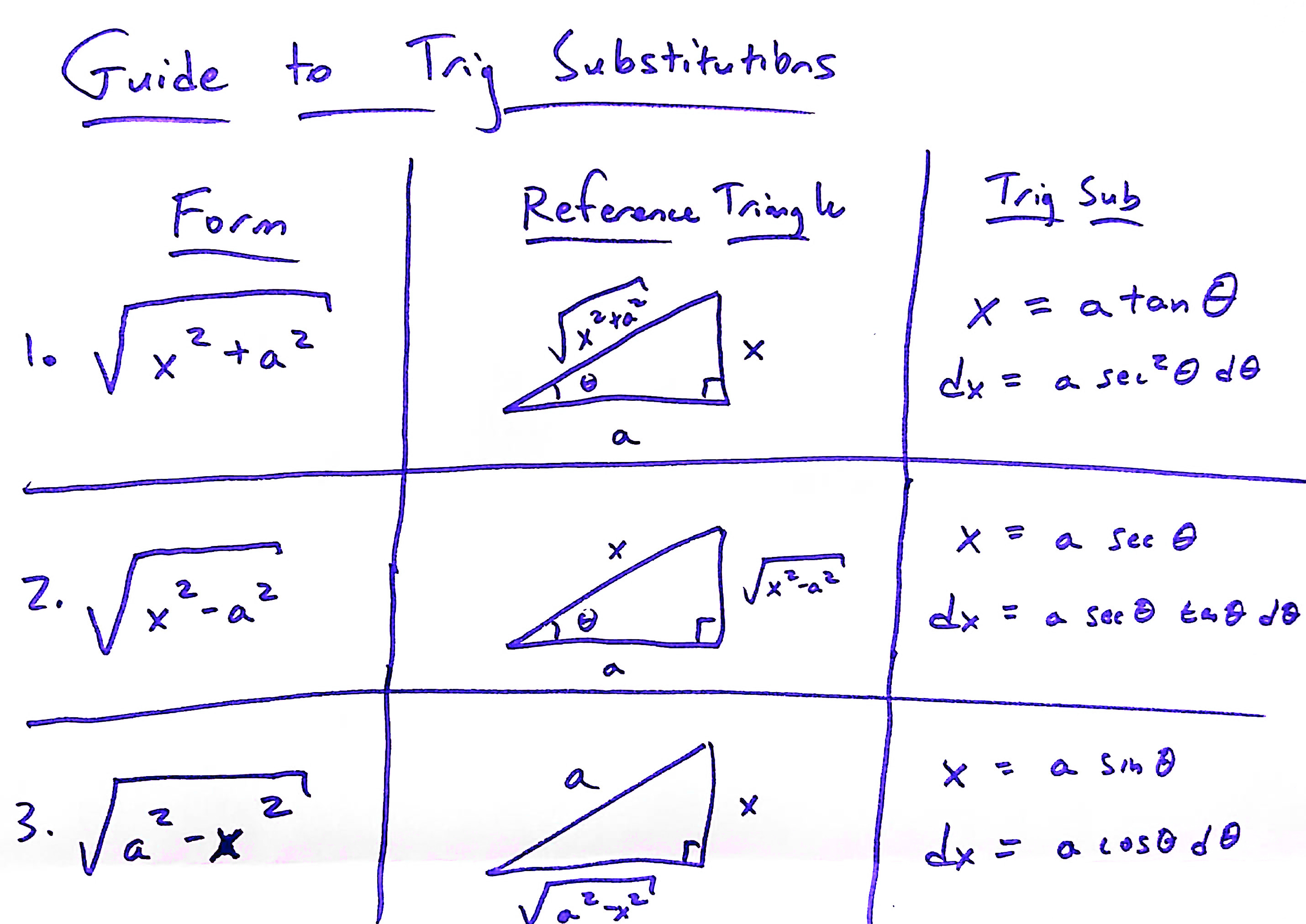
Today we talked about trigonometric substitutions. We did the following examples:

1. \(\displaystyle \int \frac{dx}{(x^2+1)^{3/2}}\).

2. \(\displaystyle \int \frac{1}{\sqrt{4-x^2}} \, dx\). (https://youtu.be/EV5dhv0A2wU)

3. \(\displaystyle \int \frac{\sqrt{x^2-9}}{x} \, dx\). (https://youtu.be/yF1JKcEMWRA)

Here is a table which summarizes all of the possible trig substitutions:

Thursday, Feb 23

Today we went over Homework 6. We also did the following example:

1. \(\displaystyle\int \sqrt{1-x^2} \, dx\)

To finish that problem we had to use both the half-angle formulas and the double angle formulas (which are on the formula sheet).

Friday, Feb 24

Today we introduced the partial fraction decomposition. This is an algebra technique that helps integrate rational functions.

1. \(\displaystyle \int \frac{3x-8}{x^2-4x-5} \, dx\). (https://www.youtube.com/watch?v=HZTv4zCgEnA)

2. \(\displaystyle \int \frac{1}{P(1-P)} \, dP\).

Partial fractions works for any rational function where the degree of the numerator (top) is less than the degree of the denominator (bottom) and the denominator factors into linear (i.e., degree 1) factors that all have different roots. If the degree of the numerator is bigger than or equal to the degree of the denominator, then use polynomial long division first.

3. \(\displaystyle \int \frac{x^3 + x}{x-1} \, dx\).

Week 7 Notes

Tentative Schedule

Monday, Feb 27

We finished partial fractions with these examples:

1. \(\displaystyle\int \frac{x-5}{-2x+2} \, dx\). (https://youtu.be/5j81gyHn9i0)

2. \(\displaystyle \int \frac{x^4-5x^2+4x}{x^2-4} \, dx\).

3. \(\displaystyle\int \frac{4x+9}{(x-1)(x+1)(x+4)} \, dx\). (https://youtu.be/hnIs8uwAT3U)

4. \(\displaystyle\int \frac{6x^2 - 19x + 15}{(x-1)(x-2)^2} \, dx\). (https://youtu.be/A52fEdPn9lg)

Wednesday, Mar 1

Today we switched from integrals to limits. We will be using limits a lot in the next few weeks, so we need a fast way to compute them. One option that works frequently (but not always) is L’Hospital’s rule.

1. \(\displaystyle \lim_{x \rightarrow 0} \frac{\sin x}{x}\). (https://youtu.be/PdSzruR5OeE)

2. \(\displaystyle \lim_{x \rightarrow 5^+} \frac{x}{x-5}\). (You can’t use L’Hospital’s rule here! Why not?)

3. \(\displaystyle \lim_{x \rightarrow \infty} \frac{x^2}{e^x}\). (https://youtu.be/Gh48aOvWcxw)

4. \(\displaystyle \lim_{x \rightarrow \infty} \frac{\ln x}{1-x}\).

5. \(\displaystyle \lim_{x \rightarrow \pi^+} \frac{\sin x}{1-\cos x}\). (Watch out, this one isn’t L’Hospital’s rule either!)

6. \(\displaystyle \lim_{x \rightarrow \infty} \frac{3x^{8}-4x^{7}+3x^{4}-5x}{2x^{7}+5x^{5}-3x+12}\) (Hint: The key to this one is to factor out the highest power of \(x\) in the numerator & denominator).

In addition to the indeterminant forms \(\frac{\infty}{\infty}\) and \(\frac{0}{0}\), there are other indeterminant forms that come up when working with limits. These include: \[0 \cdot \infty, ~ \infty - \infty, ~ 0^0, ~ 1^\infty, ~ 0^\infty\] Here are some ideas on how to deal with these when they pop up in limit calculations:

7. \(\displaystyle \lim_{x \rightarrow 0^+} x \ln x\). Hint: re-write the problem as \(\displaystyle \lim_{x \rightarrow 0^+} \dfrac{\ln x}{x^{-1}}\) so you can apply L’Hospital’s rule.

8. \(\displaystyle \lim_{x \rightarrow \tfrac{\pi}{2}^-} (\sec x - \tan x)\). Hint: combine the secant and tangent into one fraction by switching to sines and cosines.

Thursday, Mar 2

Today we went over Homework 7 and we did this example in class:

1. \(\displaystyle \lim_{n \rightarrow \infty} \left(1+ \frac{r}{n} \right)^n\) where \(r\) is any constant. Hint, let \(\displaystyle A = \lim_{n \rightarrow \infty} \left(1+ \frac{r}{n} \right)^n\) and take the natural log of both sides.

Friday, Mar 3

Today we talked about improper integrals which are integrals involving infinity (either in the bounds, or because of a vertical asymptote). You deal with these just like any other definite integral, except you might have to calculate a limit to find the answer. We did several examples:

1. \(\displaystyle \int_1^{\infty} \frac{1}{x^2} \, dx\). This one turns out to just be 1, which illustrates a very important idea: The area under an infinite curve can still be finite!

2. \(\displaystyle \int_2^3 \frac{1}{\sqrt{x-2}} \, dx\). You could integrate this one without even realizing that it is technically an improper integral. But if you look at the graph, you’ll see why it counts as an improper integral.

3. \(\displaystyle \int_2^\infty \frac{1}{x} \, dx\).

4. \(\displaystyle \int_{-\infty}^0 x e^{x} \, dx\).

If the value of the integral is a finite number, we say it converges. Otherwise, it diverges. An improper integral can diverge for two reasons. It might have infinite area, or there might not be one number that the area converges to (which is why \(\displaystyle \int_0^{\infty} \sin x \, dx\) diverges).

5. For what values of \(p\) does the integral \(\displaystyle \frac{1}{x^p} \, dx\) converge? Answer, \(p > 1\). (This is known as the \(p\)-test).

Week 8 Notes

Tentative Schedule

Monday, March 13

We started with this warm-up problem:

1. \(\displaystyle\int_e^\infty \frac{1}{x (\ln x)^3}\) (https://youtu.be/9WzQJD3j14A)

2. \(\displaystyle\int_0^\infty \sin x \, dx\) (https://youtu.be/ol9iqccSS1o)

We talked about the comparison test for integrals. If \(f(x)\) and \(g(x)\) are nonnegative functions and \(f(x) \le g(x)\), then \(\int f \le \int g\). This has two consequences:

• If the bigger function has a finite integral, then the smaller integral must be finite too.

• If the smaller function has an infinite integral, then so does the bigger one.

3. Compare the integrals \(\displaystyle \int_e^\infty \frac{1}{x \ln x} \, dx\) and \(\displaystyle \int_e^\infty \frac{1}{\ln x} \, dx\). One of these integrals is easy if you make the u-subsitution \(u = \ln x\). Does that integral converge? What about the other integral? Can you use the comparison test here?

4. Use the comparison test to show that \(\displaystyle \int_{\pi}^\infty \left( \frac{\sin x}{x} \right)^2 \, dx\) converges.

5. Does \(\displaystyle\int_1^{\infty} \frac{1}{x+e^x} \, dx\) converge or diverge? (https://youtu.be/dvCeQFRHyww)

6. Show that \(\displaystyle\int_1^\infty e^{-x^2} \, dx\) converges. (https://youtu.be/SYHoI5g8r4Q)

Wednesday, Mar 15

Today we looked at two applications of integrals. First we looked at finding areas between curves. We did these two examples:

1. Find the area between \(y = 2-x^2\) and the line \(y = x\). (https://youtu.be/x4Yp-UF4vvI)

2. Find the area between \(y = \sin x\) and \(y = \cos x\) (https://youtu.be/9FBIbttJM1A).

Then we discussed how to use integrals to find volumes. We started with the problem of finding the volume of a pyramid, and came up with the central idea: that the volume of a solid is the integral of the areas of its cross sections.

\[\text{Volume} = \int \text{Area} \, dx.\]

If the cross sections are disks, this formula becomes \(V = \displaystyle \int \pi r^2 \, dx\).

1. Find the volume of a square pyramid if the base is 100 meters by 100 meters, and the height is 50 meters.

2. Find the volume of the solid formed by revolving the region between \(y = \sqrt{x}\) and the x-axis from \(x=0\) to \(x=4\) around the \(x\)-axis.

3. Find the volume of a sphere with radius \(R\) by revolving \(y = \sqrt{R^2 - x^2}\) around the x-axis. (https://youtu.be/QLHJl2_aM5Q).

Week 9 Notes

Tentative Schedule

Monday, Mar 20

Today we did some more volume computations. We did this warm-up problem:

1. Use the disk method to find the volume of a cone that is \(h\) units tall and has a base radius of \(R\) units.

Next, we did an example of a hollow shape. To get the volume, you use the washers method since the cross sections look like flat washers. The formula for the washers method is:

\[ V= \int \pi R^2 - \pi r^2 \, dx ~(\text{or } dy)\]

2. Find the volume of the region between \(y = \sqrt{x}\) and \(y= x\) revolved around the x-axis. (https://youtu.be/vhMl755vR5Q)

Another method for finding volumes of revolution is the shells method. Here is a video explanation of the shells method. We did these examples in class.

3. Find the volume of the region under \(\cos(x^2)\), \(0 < x < \frac{\pi}{2}\), revolved around the y-axis. (https://youtu.be/EX0rslFIL18)

4. Find the volume of the region under \(y = x(x-1)^2\) from \(x=0\) to 1 revolved around the y-axis (https://youtu.be/cxj0OfZTWEo)

5. Find the volume of the region under \(y = e^{-x^2}\) from \(x=0\) to \(\infty\) revolved around they y-axis. (https://youtu.be/CiXME1u-oyU)

Wednesday, Mar 22

Today we talked about how to find the length of a curve using integrals. There are two approaches. For a function with an explicit formula \(y = f(x)\), use:

\[\text{Length} = \int_a^b \sqrt{1+(y')^2} \, dx.\]

For functions with a parametric formula where both the x and y coordinates are functions of a third parameter \(t\), use:

\[\text{Length} = \int_a^b \sqrt{(dx/dt)^2+(dy/dt)^2} \, dt.\]

This formula has a nice interpretation if \(t\) represents time. Then \((dx/dt)\) is the horizontal velocity, \((dy/dt)\) is the vertical velocity, and \(\displaystyle \sqrt{(dx/dt)^2+(dy/dt)^2}\) is the speed of the object. Then distance traveled is the integral of speed with respect to time.

1. Arc length of \(y = x^{3/2}\) from \(x=0\) to \(x = \tfrac{32}{9}\). (https://youtu.be/OhISsmqv4_8)

2. Arc length of parametric curve \(x=\cos(t)\), \(y = \sin(t)\) from \(t=0\) to \(t=\frac{\pi}{2}\). (https://youtu.be/F3KyoI26fKI)

3. Arc length of \(x = 2+6t^2\) and \(y = 5+4t^3\) when \(0 \le t \le \sqrt{8}\). (https://youtu.be/X8N21DrWmjU)

4. Write down an integral that represents the length of the parabola \(y = x^2\) from \(x = -2\) to \(x=2\).

3. Write down an integral that represents the perimeter of the ellipse with parametric equations \(x(t) = 2 \cos t\), \(y(t) = \sin t\). Then use a Riemann sum with \(N=1000\) rectangles to approximate the integral.

Friday, Mar 24

Today we talked about work and energy. For a variable force \(F= F(x)\), work is the integral of force with respect to distance: \[W = \int F \, dx.\]

We did the following examples:

1. A force of 50 lbs. is needed to stretch a spring 5 inches longer than its natural length. How much work is required to stretch it 10 inches beyond its natural length? (https://youtu.be/TLw8xbmnY3c)

2. A spring has force \(F = 10 x\) where \(x\) is the amount the spring is compressed (in meters) and the force is in Newtons. Find the work needed to compress the spring 1 meter?

3. If the compressed spring in the last problem pushes a 1 kg object along a slippery surface so that all of the potential energy of the spring is converted to kinetic energy of the object, then how fast will the object be moving after the spring pushes it? (Hint: recall that kinetic energy is \(\frac{1}{2}mv^2\).)

4. A 50 lb bucket will be raised from ground level to a height of 10 feet. The bucket is attached by a heavy chain (weighing one pound per foot) to a pulley 20 feet off the ground. How much work will it take to lift the bucket? (https://youtu.be/QA5mvSx5idE)

5. How much work is needed to pump water into a cylindrical tank that is 10 meters above the ground and is 3 meters tall with radius 1 meter? To solve this problem use the alternative formula for work: \[W = \int x \, dF\] where \(dF\) is a the weight of a slice of water: \[dF =(\text{Weight Density})(\text{Volume})=(\text{Weight Density})(\pi r^2 \, dx) \] and the weight density of water is 9800 Newtons per meter cubed.

6. How much work is needed to pump all of the water out of a conical pool that has a radius of 4 meters at the surface and is 10 meters deep, assuming that the initial water level is 8 meters deep? (Recall that the weight density of water is 9800 Newtons per meter cubed). (https://youtu.be/Ab0omZH2fFc)

Week 10 Notes

Tentative Schedule

Monday, Mar 27

Today we talked about infinite series which is an infinitely long sum of numbers. This is very different than what we’ve been doing with integrals, so I would recommend reading the introduction to Chapter 10 in the book.

Before doing any calculations, we started with three example infinite series:

1. Zeno’s series \(\displaystyle \frac{1}{2}+\frac{1}{4}+\frac{1}{8} + \frac{1}{16} + \ldots = 1\).

2. Grandi’s series \(\displaystyle 1 + (-1) + 1 + (-1) + 1 + (-1) + \ldots = DNE\).

3. Harmonic series \(\displaystyle 1 + \frac{1}{2} + \frac{1}{3} + \frac{1}{4} + \frac{1}{5} + \ldots = \infty\).

Then we talked about geometric series, which have the formula:

\[a + ax + ax^2 + ax^3 + ax^4 + \ldots = \frac{a}{1-x}\]
as long as the common ratio \(x\) satisfies \(|x| < 1\). Geometric series diverge if \(|x| \ge 1\), which means the infinite sum does not make sense.

We did the following examples in class:

1. What is the sum of \(\displaystyle 1+ \frac{2}{3}+\frac{4}{9}+\frac{8}{27} + \frac{16}{81} + \ldots\)?

2. Find the sum of \(\displaystyle\sum_{n=1}^\infty \frac{(-3)^{n-1}}{4^n}\). (https://youtu.be/uebsyi1Jigw)

3. If the sides of the outer square are both 2 meters long, find the total area of the darker squares:

4. Convert the repeating decimal \(0.36363636\ldots\) to a geometric series and then a reduced fraction.

5. If \(f(x) = 1 + x + x^2 + x^3 + x^4 + \ldots\), what is \(f(-x^2)\)?

Wednesday, Mar 29

Today we talked about what it means for an infinite series to converge. A series converges if the limit of its partial sums is a finite number. For a geometric series \(1+x+x^2 + x^3 + \ldots\), this happens if and only if \(|x| < 1\).

Then we talked about converting series that are written in term-by-term notation (like \(\tfrac{1}{2} + \frac{1}{4} + \frac{1}{8} + \frac{1}{16} + \ldots\)) into summation notation with a \(\Sigma\)-symbol. There are certain common patterns to watch out for:

• Arithmetic patterns When you add the same amount each step. A formula for this pattern is \[a + bn\] where \(a\) is the first term and \(b\) is the step size.

• Geometric patterns When you multiply by the same amount each step.
  \[a r^n\] where \(a\) is the first term and \(r\) is the common ratio (the common amount you multiply by).

• Alternating patterns If the terms alternate between positive and negative, you can write a formula for this by including a factor of \((-1)^n\).

We did the following examples (since these aren’t in most textbooks, I’ve included solutions too.).

1. Express the series \(4 - \frac{4}{3} + \frac{4}{5} - \frac{4}{7} + \frac{4}{9} - \ldots\) using \(\Sigma\)-notation.
   Solution

   This series has alternating terms and it has an arithmetic pattern in the denominator. To make the terms alternate, multiply by \((-1)^n\). The numerator is always 4, and the denominator starts at 1 and increases by 2 every step, so a formula for that arithmetic pattern would be \((1+2n)\). Putting it all together, we get: \[\sum_{n=0}^\infty \frac{(-1)^n \cdot 4}{(1+2n)}.\]

After this example we paused to talk about the definition of convergence: An infinite series converges if the limit of its partial sums exists, otherwise it diverges. We proved that a geometric series \(\sum_{n=0} a r^n\) converges when \(|r|<1\). Here is a video that goes over that proof. Then we did more examples of recognizing patterns.

2. Express the series \(\frac{5}{3} + \frac{7}{4} + \frac{9}{5} + \frac{11}{6} + \ldots\) in \(\Sigma\)-notation.
   Solution

   This time, both the numerator and denominator follow arithmetic patterns, so the solution is: \[\sum_{n=0}^\infty \frac{(5+2n)}{(3+n)}.\]

3. Re-write the following series in \(\Sigma\)-notation: \(1 - \frac{4}{3} + \frac{9}{9} - \frac{16}{27} + \frac{25}{81} - \ldots\).
   Solution

   Here the pattern is alternating, and the numbers on the top are perfect squares. So the pattern on top looks like \((-1)^n n^2\), but that doesn’t come out quite right. If the sum starts at \(n=0\), you need \((-1)^n (n+1)^2\) to get the top right. The pattern on the bottom is geometric with common ratio 3, so the solution is: \[\sum_{n=0}^\infty \frac{(-1)^n (n+1)^2}{3^n}.\]

Working with Factorials

Another pattern that is common with series is the factorial. Some important things to know include the fact that \(0! = 1\), and that expressions with factorials in both the numerator and denominator can be simplified by canceling the factors inside. For example, simplify the following expressions (without a calculator):

4. \(\displaystyle \frac{10!}{7!}\).

5. \(\displaystyle \frac{5! \, 4!}{(3!)^2}\).

6. \(\displaystyle \frac{(3n+3)!}{(3n)!}\).

Friday, Mar 31

Today we looked at some things you can do with geometric series that have a variable x. We followed Section 10.1 from the book very closely, so I recommend reading that section carefully too.

1. Find the derivative of \(\displaystyle 1 + x + x^2 + x^3 + \ldots = \frac{1}{1-x}\).
   

2. Multiply the series: \[\left(1 + x + x^2 + x^3 + \ldots \right) \left( 1 + x + x^2 + x^3 + \ldots \right).\]

3. Subtract the series \[\left(1 + x + x^2 + x^3 + \ldots \right) - \left(1 - x + x^2 - x^3 + \ldots \right).\]

4. Integrate the series \(1 - x + x^2 - x^3 + \ldots\). Use this to find an infinite series for \(\ln(1+x)\).

5. Substitute \(x^2\) in place of \(x\) in the series \(1+x+x^2+x^3 + \ldots.\)

6. Integrate the previous series to find an infinite series for \(\arctan x\).

Week 11 Notes

Tentative Schedule

Wednesday, Apr 5

Here is a simple idea that is pretty obvious: an infinite sum cannot converge unless the terms in the sum are getting closer and closer to zero. That’s one reason that Grandi’s series (\(1-1+1-1+1-1+1-\ldots\)) cannot converge. This simple idea is called the divergence test. Unfortunately, you can’t turn it around and say that a series with terms getting closer & closer to zero will converge. That isn’t true.

A p-series is a series of the form:

\[\sum_{n = 1}^\infty \frac{1}{n^p} = 1 + \frac{1}{2^p} + \frac{1}{3^p} + \frac{1}{4^p} + \ldots.\]

The special case when \(p = 1\) is called the harmonic series.

Integral Test. A series \(\displaystyle\sum_{n = 1}^\infty f(n)\) with positive terms that are given by a decreasing function \(f(n)\) converges if and only if the integral \(\int_1^\infty f(x) \, dx\) converges.

We used the integral test to show that p-series converge if \(p > 1\) and they diverge otherwise. This is called the p-test for convergence. We finished with the following examples:

1. Show that the series \(2+ \frac{4}{3} + \frac{6}{9} + \frac{8}{27} + \frac{10}{81} + \ldots\) converges by finding a larger simpler series that also converges.
   
   Solution

   First we converted the series to \(\Sigma\)-notation. We got \[\displaystyle \sum_{n=0}^\infty \frac{2+2n}{3^n}.\]
   To find a larger series, we can either make the numerator larger or the denominator smaller. A good option here to to notice that \(2^n\) is bigger than \(2+2n\) for all \(n\) bigger than one. So \[\sum_{n=0}^\infty \frac{2+2n}{3^n} \le \sum_{n=0}^\infty \frac{2^n}{3^n}.\] The series on the right-side is geometric with common ratio \(x = \frac{2}{3}\), so it converges. Therefore the smaller series on the left-side must also converge.

This is an example of the comparison test which works the same for infinite series as it does for integrals.

2. Use the integral test to show that the series \(\displaystyle\sum_{n = 2}^\infty \frac{1}{n(\ln n)^2}\) converges.

3. Use the comparison test to show that \(\displaystyle\sum_{n = 0}^\infty \frac{1}{n!}\) converges.

Friday, Apr 7

Today we went off on a bit of a tangent and talked about the series from Problem 3 in HW11. The answer to problem 3 is the series:

\[\ln\left(\frac{1+x}{1-x} \right) = 2x + \frac{2}{3}x^3 + \frac{2}{5} x^5 + \frac{2}{7} x^7 + \ldots.\]

We substituted \(x = \frac{1}{2}\) to get an infinite series for \(\ln(3)\).

1. Write the series above with x = 1/2 in term-by-term notation.

2. Re-write the series in Σ-notation.

3. How can you tell that this series converges?

4. Use a computer to add the first 10 terms of the series. How accurate is the approximation for \(\ln(3)\)?

Week 12 Notes

Tentative Schedule

Monday, Apr 10

Alternating series have terms that alternate between positive and negative. They can be expressed as

\[\sum_{n=0}^\infty (-1)^n b_n\] where \(b_n\) is always positive.

Alternating series will converge if the following conditions are satisfied:

• \(\lim_{n \rightarrow \infty} b_n = 0\) and
• \(b_{n+1} \le b_n\) for every \(n\).

These conditions are called the alternating series test. If an alternating series meets the conditions of the alternating series test, then you can estimate the error in a partial sum using the formula:

\[\text{Error} = |S_\infty-S_n| \le b_{n+1}\]

A good example of an alternative series is the alternating harmonic series: \(1 - \frac{1}{2} + \frac{1}{3} - \frac{1}{4} + \frac{1}{5} - \ldots\). Unlike the regular harmonic series which diverges, the alternative harmonic series converges by the alternating series test.

For each of the following, write out the first 4 terms of the alternating series, and determine whether it converges or diverges. How many terms would you need to make the error less than \(10^{-6}\)?

1. \(\sum_{n=0}^\infty \frac{ (-1)^n }{n!}\)

2. \(\sum_{n=1}^\infty (-1)^n / \sqrt{n}\)

A power series is like an infinite degree polynomial. A power series has the form \[\sum_{n=0}^\infty a_n (x-c)^n = a_0 + a_1 (x-c) + a_2 (x-c)^2 + a_3 (x-c)^3 + \ldots\] where the numbers \(a_n\) are called the coefficients and the number \(c\) is called the center of the power series. All power series have a radius of convergence \(R\). When \(|x-c| < R\), the series converges, and when \(|x-c| > R\), the series diverges. At the endpoints, \(x = c \pm R\), the series might converge or diverge. To find the radius of convergence, use the ratio test formula: \[R = \lim_{n \rightarrow \infty} \frac{|a_n|}{|a_{n+1}|}.\]

3. Find the radius of convergence for the power series \(1 + x + x^2 + x^3 + \ldots\).

4. Find the interval of convergence for the power series \(\displaystyle \sum_{n = 0}^\infty \frac{x^n}{n!}\).

Wednesday, Apr 12

Today we introduced Taylor series and Maclaurin series. A Taylor series is a power series for a function \(f(x)\) that can be calculated by finding all of the derivatives of the function when \(x=c\):

\[f(x) = \sum_{n=0}^\infty \frac{f^{(n)}(c)}{n!} (x-c)^n\]

In this formula, \(f^{(n)}(c)\) is the n-th derivative of \(f\) at the point \(x=c\) (recall that \(c\) is the center of the power series. Usually \(c=0\)). When the center is \(c=0\), we call the series a Maclaurin series sometimes (but it is still a Taylor series too).

We did the following examples in class:

1. Find the Maclaurin series for \(f(x) = \sin x\) by making a table of derivatives and finding the pattern. (https://youtu.be/8dMLK2Wueaw)

2. Find the radius of convergence for the Maclaurin series for \(\sin x\) using the formula \(R = \displaystyle \lim_{n \rightarrow \infty} \frac{|a_n|}{|a_{n+1}|}\).

3. According to the Maclaurin series, \(\sin(1) \approx 1 - \frac{1}{3!} + \frac{1}{5!} - \frac{1}{7!} + \frac{1}{9!}.\) Estimate the worst case error in this approximation.

4. Find the Maclaurin series for \(f(x) = e^x\) by making a table of derivatives and finding the pattern. (https://youtu.be/JYQqml4-4q4)

5. Find the Taylor series for \(f(x) = \ln x\) centered at \(c = 1\).

Friday, Apr 14

We reviewed Homework 12 before the quiz. After the quiz, we did the following:

1. Use power series to find an infinite series for the integral \(\displaystyle\int_0^\pi \frac{\sin x}{x} \, dx\).

2. How many terms of the infinite series would you need to approximate the answer accurate to eight decimal places (i.e., with error less than \(10^{-8}\))?

Since the answer to part 1 was an alternating series, we could just use the alternating series error formula.

Sometimes with Taylor series applications you get series that are not alternating. So we need another method to estimate error. For example, we ended with this question:

3. Find the 5th degree Maclaurin polynomial for \(e^x\) and use it to approximate \(e\).

Week 13 Notes

Tentative Schedule

Monday, Apr 17

Today we introduced

Taylor’s Remainder Theorem. If \(f\) is a function with \(N+1\) derivatives between \(x\) and \(c\) and \(f^{(N)}\) is continuous at \(x\) and \(c\), then there exists \(z\) between \(x\) and \(c\) such that the remainder of \(f(x) - P_N(x)\) is \[R_N(x) = \frac{f^{(N+1)}(z)}{(N+1)!} (x-c)^{N+1}.\]

1. Find the 2nd degree Maclaurin polynomial for \(\cos x\) and use Taylor’s remainder theorem to estimate the error in the approximation \(\cos x \approx P_2(x)\).

2. The fifth degree Maclaurin polynomial approximation for \(e^1\) is \[e^1 \approx 1 + \frac{1}{1!} + \frac{1}{2!} + \frac{1}{3!} + \frac{1}{4!} + \frac{1}{5!} = 2.71\overline{6}.\] Find an expression for the remainder function \(R_5(x)\) for the Maclaurin series for \(e^x\) and use it to estimate the error in the approximation above (when \(x=1\)).

3. Find the 2nd degree Taylor polynomial for \(f(x) = \sqrt[3]{x}\) centered at \(c=8\) and find an expression for the remainder \(R_2(x)\).

Wednesday, Apr 19

Today we looked at applications of Taylor series.

1. First I showed how to solve the differential equation \(y'' = -y\) with initial conditions \(y(0) = 4\), \(y'(0) = -3\) by figuring out a pattern for the higher derivatives and using a Taylor series.

Then we did the applications in this handout:

• Taylor Series Applications

Week 14 Notes

Tentative Schedule